R and RStudio - Basics
Day 1
January 15, 2024
Difference between R and RStudio

![]()
R is the programming language and the program that does the actual work
- Can be used with many different programming environments
RStudio is the integrated development environment (IDE)
- Provides an interface to R
- Specifically built around R code
- Execute code
- Syntax highlighting
- File and project management
- …
Difference between R and RStudio
![]()

Summary
You can use R without RStudio but RStudio without R would be of little use
Introduction to RStudio
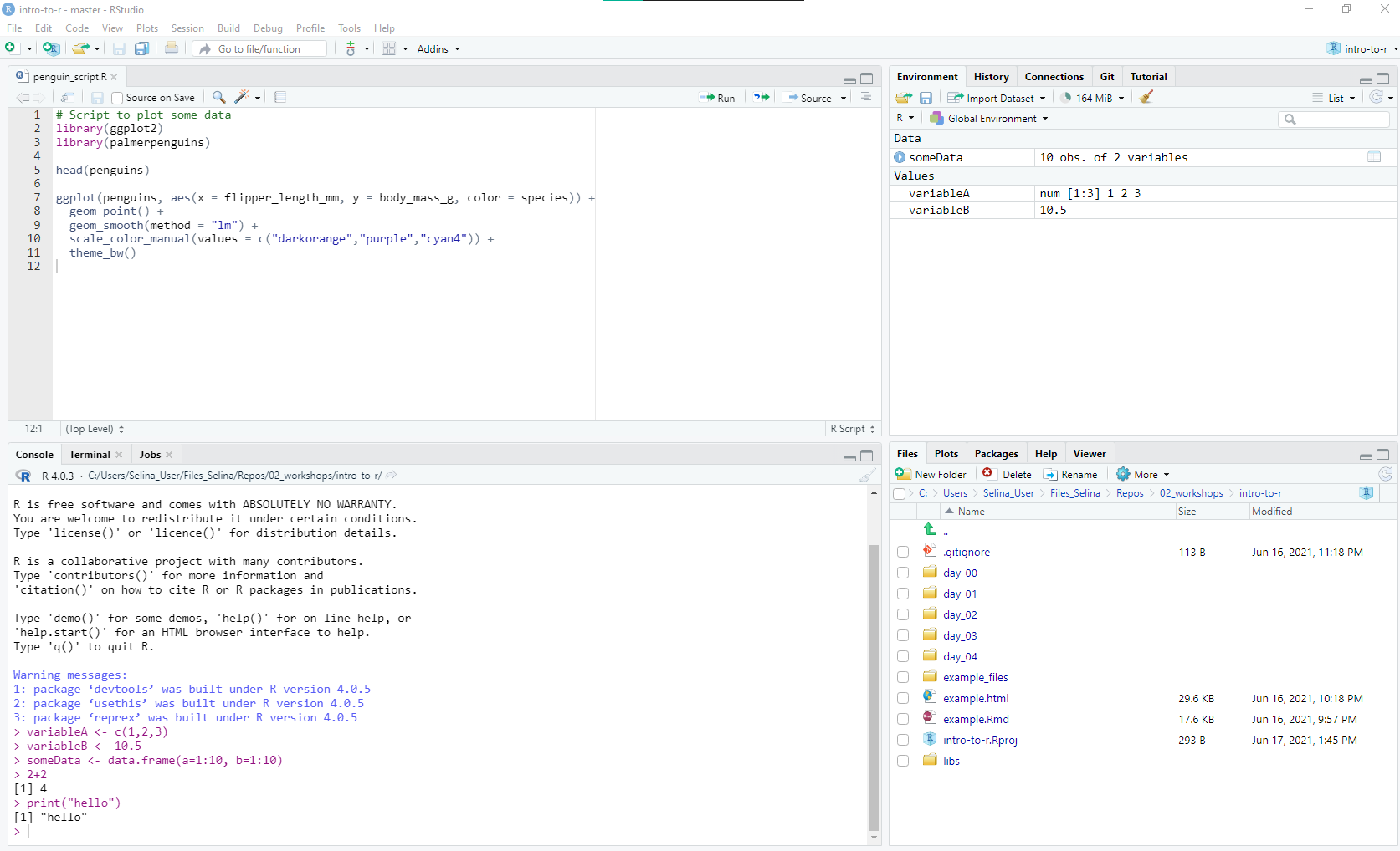
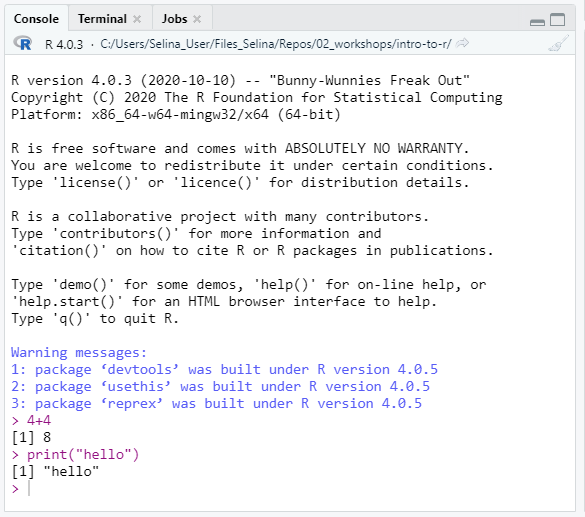
Console pane
Execute R code
Output from R code in scripts is printed there
Type a command into the console and execute with
Enter/Return
Tip
Use arrow keys to bring back last commands
Script pane
-
Write scripts with R code
Scripts are text files with R commands (file ending
.R)Use scripts to save commands for reuse
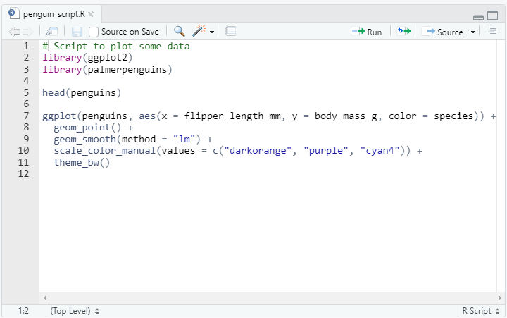
Script pane
- Create a new R script:
File -> New File -> R Script - Save an R script:
File->Save (Ctrl/Cmd + S) - Run code line by line with Run button (Ctrl+Enter/Cmd+Return)
- You can open multiple scripts
Summary
Use scripts for all your analysis and for commands that you want to save.
Use console for temporary commands, e.g. to test something.
Environment pane
Shows objects currently present in the R session
Is empty if you start R

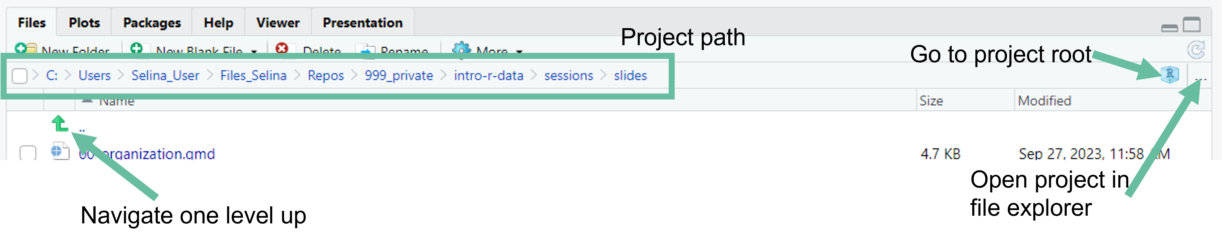
Files pane
Similar to Explorer/Finder
-
Browse project structure and files
- Find and open files
- Create new folders
- Delete files
- Rename files
- …
Practical if you don’t want to switch between File Explorer and RStudio all the time
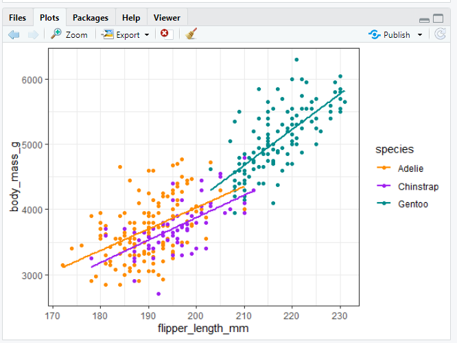
Plot pane
- Plots that are created with R will be shown here
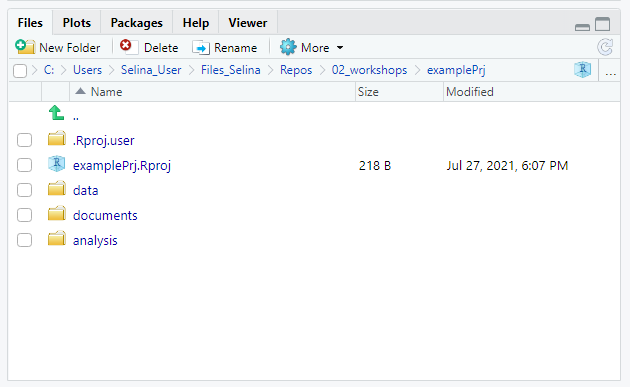
Create an RStudio project
Create a project from scratch:
- File -> New Project -> New Directory -> New Project
- Enter a directory name (this will be the name of your project)
- Choose the Directory where the project should be initiated
- Create Project
RStudio will now create and open the project for you.
Navigate an RStudio project
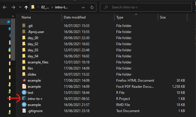
Open a project from outside RStudio
To open an RStudio project from your file explorer/finder, just double click on the .Rproj file
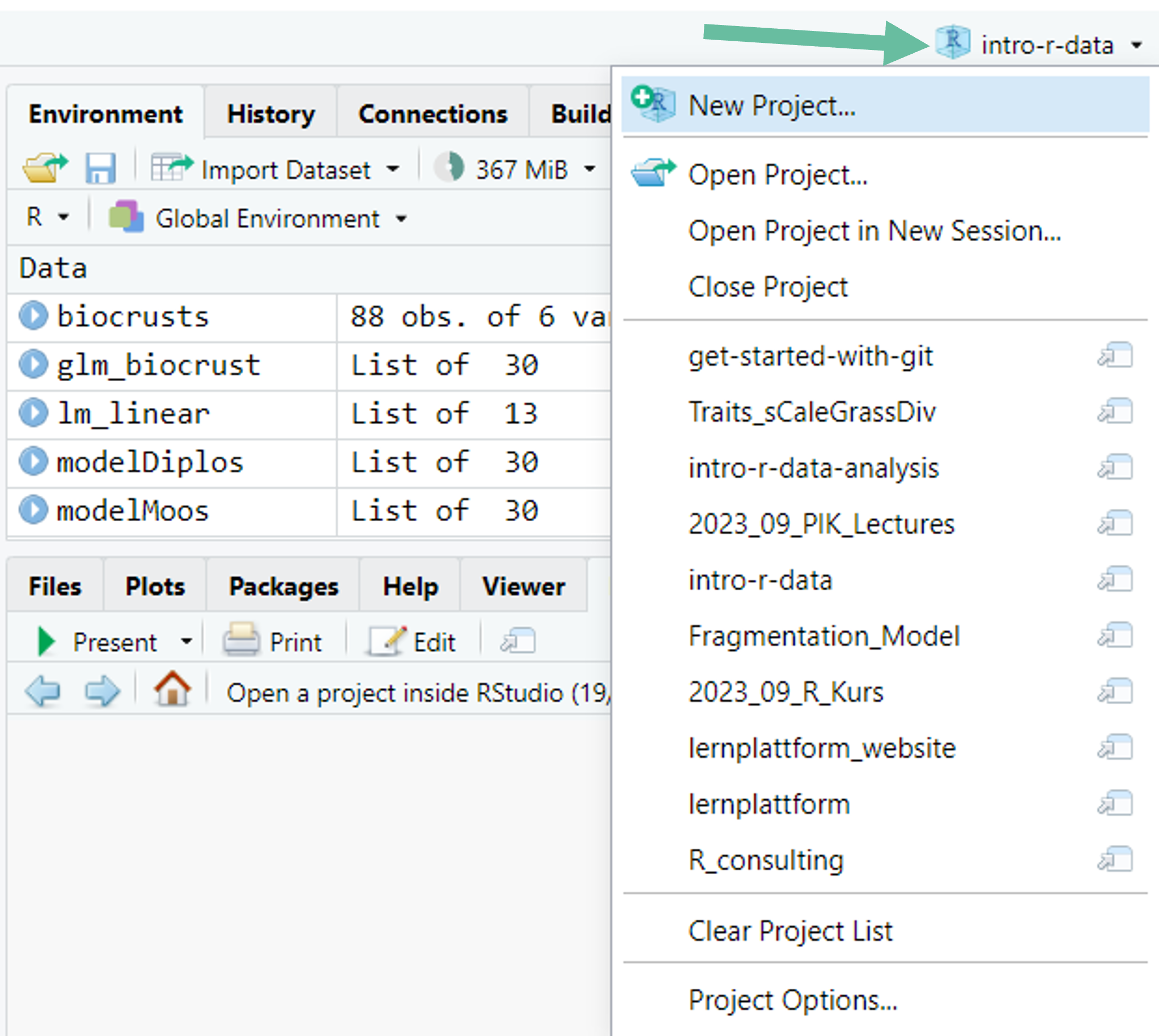
Open a project inside RStudio
To open an RStudio project from RStudio, click on the project symbol on the top right of R Studio and select the project from the list.
Basic R Syntax
- Whitespace does not matter
# this
data<-read_csv("data/my-data.csv")

# is the same as this

data <-
  read_csv(    "data/my-data.csv"   )
There are good practice rules however -> More on that later
-
RStudio will (often) tell you if something is incorrect
- Find
![]() on the side of your script
on the side of your script
- Find
 on the side of your script
Vectors
Vectors are data structures that are built on top of atomic data types.
Imagine a vector as a collection of values that are all of the same data type.

Image from Advanced R book
Comments in R
#is a commentCtrl/Cmd + Shift + R)