Data handling with dplyr

Day 2

Jonas Vollhüter

Freie Universität Berlin @ Theoretical Ecology

January 16, 2024

1 Data transformation

1.1 Data transformation

Data transformation is an important step in understanding the data and preparing it for further analysis.

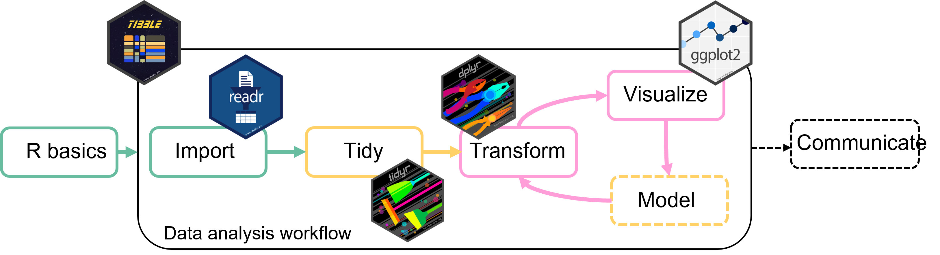
We can use the tidyverse package dplyr for this.

1.2 Data transformation

With dplyr we can (among other things)

Filter data to analyse only a part of it
Create new variables
Summarize data
Combine multiple tables
Rename variables
Reorder observations or variables

To get started load the package dplyr:

library(dplyr) # or: library(tidyverse)

1.3 Dplyr basic vocuabulary for data manipulation

filter() picks observations (rows) based on their values
select() picks variables (columns) based on their names
mutate() adds new variables based on existing ones
summarize() combines multiple values into a single summary value

Perform any of these operations by group

1.4 Dplyr basic vocabulary

All of the dplyr functions work similarly:

First argument is the data (a tibble)
Other arguments specify what to do exactly
Return a tibble

1.5 Example data

Soybean production for different use by year and country.

soybean_use <- readr::read_csv('https://raw.githubusercontent.com/rfordatascience/tidytuesday/master/data/2021/2021-04-06/soybean_use.csv')
soybean_use

# A tibble: 9,897 × 6
   entity code   year human_food animal_feed processed
   <chr>  <chr> <dbl>      <dbl>       <dbl>     <dbl>
 1 Africa <NA>   1961      33000        6000     14000
 2 Africa <NA>   1962      43000        7000     17000
 3 Africa <NA>   1963      31000        7000      5000
 4 Africa <NA>   1964      43000        6000     14000
 5 Africa <NA>   1965      34000        6000     12000
 6 Africa <NA>   1966      41000        6000      2000
 7 Africa <NA>   1967      47000        6000      4000
 8 Africa <NA>   1968      50000        7000      3000
 9 Africa <NA>   1969      52000        6000      6000
10 Africa <NA>   1970      52000        6000      8000
# ℹ 9,887 more rows

2 `filter()`

picks observations (rows) based on their value

Artwork by Allison Horst

2.1 Useful `filter()` helpers

These functions and operators help you filter your observations:

relational operators <, >, ==, …
logical operators &, |, !
%in% to filter multiple values
is.na() to filter missing values
between() to filter values that are between an upper and lower boundary
near() to compare floating points (use instead of == for doubles)

2.2 `filter()`

Filter rows that contain the values for Germany

filter(soybean_use, entity == "Germany")

# A tibble: 53 × 6
   entity  code   year human_food animal_feed processed
   <chr>   <chr> <dbl>      <dbl>       <dbl>     <dbl>
 1 Germany DEU    1961          0        3000   1042000
 2 Germany DEU    1962          0        3000    935000
 3 Germany DEU    1963          0        3000   1092000
 4 Germany DEU    1964          0        3000   1096000
 5 Germany DEU    1965          0        3000   1435000
 6 Germany DEU    1966          0        3000   1588000
 7 Germany DEU    1967          0        3000   1646000
 8 Germany DEU    1968          0        3000   1480000
 9 Germany DEU    1969          0        3000   1423000
10 Germany DEU    1970          0        3000   2118000
# ℹ 43 more rows

filter() goes through each row of the data and return only those rows where the value for entity is "Germany"

2.3 `filter()` + `%in%`

Use the %in% operator to filter rows based on multiple values, e.g. countries

countries_select <- c("Germany", "Austria", "Switzerland")
filter(soybean_use, entity %in% countries_select)

# A tibble: 159 × 6
   entity  code   year human_food animal_feed processed
   <chr>   <chr> <dbl>      <dbl>       <dbl>     <dbl>
 1 Austria AUT    1961          0           0         0
 2 Austria AUT    1962          0           0         0
 3 Austria AUT    1963          0           0         0
 4 Austria AUT    1964          0           0         0
 5 Austria AUT    1965          0           0         0
 6 Austria AUT    1966          0           0         0
 7 Austria AUT    1967          0           0         0
 8 Austria AUT    1968          0           0         0
 9 Austria AUT    1969          0           0         0
10 Austria AUT    1970          0           0         0
# ℹ 149 more rows

2.4 `filter()` + `is.na()`

Filter only rows that don’t have a country code (i.e. the continents etc.)

filter(soybean_use, is.na(code))

# A tibble: 1,734 × 6
   entity code   year human_food animal_feed processed
   <chr>  <chr> <dbl>      <dbl>       <dbl>     <dbl>
 1 Africa <NA>   1961      33000        6000     14000
 2 Africa <NA>   1962      43000        7000     17000
 3 Africa <NA>   1963      31000        7000      5000
 4 Africa <NA>   1964      43000        6000     14000
 5 Africa <NA>   1965      34000        6000     12000
 6 Africa <NA>   1966      41000        6000      2000
 7 Africa <NA>   1967      47000        6000      4000
 8 Africa <NA>   1968      50000        7000      3000
 9 Africa <NA>   1969      52000        6000      6000
10 Africa <NA>   1970      52000        6000      8000
# ℹ 1,724 more rows

Or the opposite: filter only the rows that have a country code with

filter(soybean_use, !is.na(code))

2.5 `filter()` + `between()`

Combine different filters:

Select rows where

the value for years is between 1970 and 1980
the value for entity is Germany

filter(soybean_use, between(year, 1970, 1980) & entity == "Germany")

# A tibble: 11 × 6
   entity  code   year human_food animal_feed processed
   <chr>   <chr> <dbl>      <dbl>       <dbl>     <dbl>
 1 Germany DEU    1970          0        3000   2118000
 2 Germany DEU    1971          0        3000   2119000
 3 Germany DEU    1972          0        5000   2271000
 4 Germany DEU    1973          0        3000   2820000
 5 Germany DEU    1974          0        3000   3704000
 6 Germany DEU    1975          0        3000   3480000
 7 Germany DEU    1976          0        1000   3453000
 8 Germany DEU    1977          0        3000   3388000
 9 Germany DEU    1978          0        3000   3647000
10 Germany DEU    1979          0        2000   3700000
# ℹ 1 more row

3 `select()`

picks variables (columns) based on their names

3.1 Useful `select()` helpers

starts_with() and ends_with(): variable names that start/end with a specific string
contains(): variable names that contain a specific string
matches(): variable names that match a regular expression
any_of() and all_of(): variables that are contained in a character vector

3.2 `select()`

Select the variables entity, year and human food

select(soybean_use, entity, year, human_food)

# A tibble: 9,897 × 3
   entity  year human_food
   <chr>  <dbl>      <dbl>
 1 Africa  1961      33000
 2 Africa  1962      43000
 3 Africa  1963      31000
 4 Africa  1964      43000
 5 Africa  1965      34000
 6 Africa  1966      41000
 7 Africa  1967      47000
 8 Africa  1968      50000
 9 Africa  1969      52000
10 Africa  1970      52000
# ℹ 9,887 more rows

Remove variables using -

select(soybean_use, -entity, -year, -human_food)

3.3 `select()` + `ends_with()`

Select all columns that end with "d"

select(soybean_use, ends_with("d"))

# A tibble: 9,897 × 3
  human_food animal_feed processed
       <dbl>       <dbl>     <dbl>
1      33000        6000     14000
2      43000        7000     17000
3      31000        7000      5000
# ℹ 9,894 more rows

You can use the same structure for starts_with() and contains().

# this does not match any rows in the soy bean data set
# but combinations like this are helpful for research data
select(soybean_use, starts_with("sample_"))

select(soybean_use, contains("_id_"))

3.4 `select()` + `any_of()`/`all_of()`

Use a character vector in conjunction with column selection

cols <- c("sample_", "year", "processed", "entity")

any_of() returns any columns that match an element in cols

select(soybean_use, any_of(cols))

# A tibble: 9,897 × 3
   year processed entity
  <dbl>     <dbl> <chr> 
1  1961     14000 Africa
# ℹ 9,896 more rows

all_of() tries to match all elements in cols and returns an error if an element does not exist

select(soybean_use, all_of(cols))

Error in `all_of()`:
! Can't subset columns that don't exist.
✖ Column `sample_` doesn't exist.

3.5 `select()` + `from:to`

Multiple consecutive columns can be selected using the from:to structure with either column id or variable name:

select(soybean_use, 1:3)
select(soybean_use, code:animal_feed)

# A tibble: 9,897 × 4
  code   year human_food animal_feed
  <chr> <dbl>      <dbl>       <dbl>
1 <NA>   1961      33000        6000
2 <NA>   1962      43000        7000
3 <NA>   1963      31000        7000
# ℹ 9,894 more rows

Be a bit careful with these commands: They are not robust if you e.g. change the order of your columns at some point.

4 `mutate()`

Adds new variables

Artwork by Allison Horst

4.1 `mutate()`

New columns can be added based on values from other columns

mutate(soybean_use,
  sum_human_animal = human_food + animal_feed
)

# A tibble: 9,897 × 7
  entity code   year human_food animal_feed processed sum_human_animal
  <chr>  <chr> <dbl>      <dbl>       <dbl>     <dbl>            <dbl>
1 Africa <NA>   1961      33000        6000     14000            39000
2 Africa <NA>   1962      43000        7000     17000            50000
3 Africa <NA>   1963      31000        7000      5000            38000
# ℹ 9,894 more rows

Add multiple new columns at once:

mutate(soybean_use,
  sum_human_animal = human_food + animal_feed,
  total = human_food + animal_feed + processed
)

4.2 `mutate()` + `case_when()`

Use case_when to add column values conditional on other columns.

case_when() can combine many cases into one.

mutate(soybean_use,
  legislation = case_when(
    between(year, 1980, 2000) ~ "legislation_1",  # case 1
    year >= 2000 ~ "legislation_2",               # case 2
    .default = "no_legislation"                   # all other cases
  )
)

# A tibble: 9,897 × 7
   entity code   year human_food animal_feed processed legislation   
   <chr>  <chr> <dbl>      <dbl>       <dbl>     <dbl> <chr>         
 1 Africa <NA>   1961      33000        6000     14000 no_legislation
 2 Africa <NA>   1962      43000        7000     17000 no_legislation
 3 Africa <NA>   1963      31000        7000      5000 no_legislation
 4 Africa <NA>   1964      43000        6000     14000 no_legislation
 5 Africa <NA>   1965      34000        6000     12000 no_legislation
 6 Africa <NA>   1966      41000        6000      2000 no_legislation
 7 Africa <NA>   1967      47000        6000      4000 no_legislation
 8 Africa <NA>   1968      50000        7000      3000 no_legislation
 9 Africa <NA>   1969      52000        6000      6000 no_legislation
10 Africa <NA>   1970      52000        6000      8000 no_legislation
# ℹ 9,887 more rows

5 `summarize()`

summarizes data

5.1 `summarize()`

summarize will collapse the data to a single row

summarize(soybean_use,
  total_animal = sum(animal_feed, na.rm = TRUE),
  total_human = sum(human_food, na.rm = TRUE)
)

# A tibble: 1 × 2
  total_animal total_human
         <dbl>       <dbl>
1    942503000  1589729000

5.2 `summarize()` by group

summarize is much more useful in combination with the grouping argument .by

summary will be calculated separately for each group

# summarize the grouped data
summarize(soybean_use,
  total_animal = sum(animal_feed, na.rm = TRUE),
  total_human = sum(human_food, na.rm = TRUE),
  .by = year
)

# A tibble: 53 × 3
    year total_animal total_human
   <dbl>        <dbl>       <dbl>
 1  1961      1503000    16994000
 2  1962      1800000    17326000
 3  1963      2060000    18667000
 4  1964      2002000    19639000
 5  1965      2162000    17796000
 6  1966      3096000    22179000
 7  1967      2818000    23282000
 8  1968      3361000    22747000
 9  1969      3084000    22212000
10  1970      2496000    24119000
# ℹ 43 more rows

5.3 `count()`

Counts observations by group

# count rows grouped by year
count(soybean_use, year)

# A tibble: 53 × 2
    year     n
   <dbl> <int>
 1  1961   178
 2  1962   178
 3  1963   178
 4  1964   178
 5  1965   178
 6  1966   178
 7  1967   178
 8  1968   178
 9  1969   178
10  1970   178
# ℹ 43 more rows

6 The pipe `%>%`

Combine multiple data operations into one command

6.1 The pipe `%>%`

Data transformation often requires multiple operations in sequence.

The pipe operator %>% helps to keep these operations clear and readable.

You may also see |> from the base R

6.2 The pipe `%>%`

Let’s look at an example without pipe:

# 1: filter rows that actually represent a country
soybean_new <- filter(soybean_use, !is.na(code))

# 2: summarize mean values by year
soybean_new <- summarize(soybean_new,
  mean_processed = mean(processed, na.rm = TRUE),
  sd_processed = sd(processed, na.rm = TRUE),
  .by = year
)

How could we make this more efficient?

6.3 The pipe `%>%`

We could do everything in one step without intermediate results by using use one nested function

soybean_new <- summarize(
  filter(soybean_use, !is.na(code)),
  mean_processed = mean(processed, na.rm = TRUE),
  sd_processed = sd(processed, na.rm = TRUE),
  .by = year
)

But this gets complicated and error prone very quickly

6.4 The pipe `%>%`

The pipe operator makes it very easy to combine multiple operations:

soybean_new <- soybean_use %>%
  filter(!is.na(code)) %>%
  summarize(
    mean_processed = mean(processed, na.rm = TRUE),
    sd_processed = sd(processed, na.rm = TRUE),
    .by = year
  )

You can read from top to bottom and interpret the %>% as an “and then do”.

6.5 The pipe `%>%`

But what is happening?

The pipe is “pushing” the result of one line into the first argument of the function from the next line.

soybean_use %>% 
  count(year)

# instead of 
count(soybean_use, year)

Piping works perfectly with the tidyverse functions because they are designed to return a tibble and take a tibble as first argument.

Tip

Use the keyboard shortcut Ctrl/Cmd + Shift + M to insert %>%

6.6 The pipe `%>%`

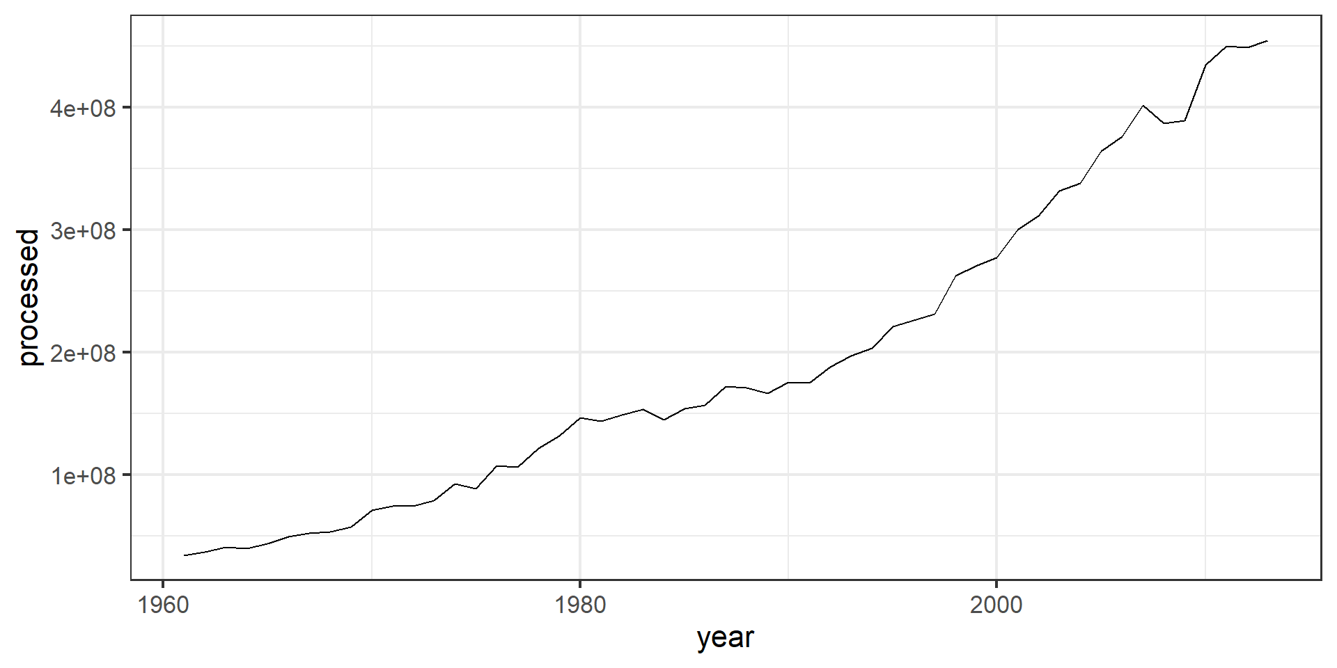
Piping also works well together with ggplot

soybean_use %>%
  filter(!is.na(code)) %>%
  select(year, processed) %>%
  summarize(
    processed = sum(processed,
      na.rm = TRUE
    ),
    .by = year
  ) %>%
  ggplot(aes(
    x = year,
    y = processed
  )) +
  geom_line()

7 Combining mulitiple tables

7.1 Combine two tibbles by row `bind_rows`

Situation: Two (or more) tibbles with the same variables (column names)

tbl_a <- soybean_use[1:2, ] # first two rows
tbl_b <- soybean_use[2:nrow(soybean_use), ] # the rest

tbl_a

# A tibble: 2 × 6
  entity code   year human_food animal_feed processed
  <chr>  <chr> <dbl>      <dbl>       <dbl>     <dbl>
1 Africa <NA>   1961      33000        6000     14000
2 Africa <NA>   1962      43000        7000     17000

tbl_b

# A tibble: 9,896 × 6
  entity code   year human_food animal_feed processed
  <chr>  <chr> <dbl>      <dbl>       <dbl>     <dbl>
1 Africa <NA>   1962      43000        7000     17000
2 Africa <NA>   1963      31000        7000      5000
# ℹ 9,894 more rows

7.2 Combine two tibbles by row `bind_rows`

Bind the rows together with bind_rows():

bind_rows(tbl_a, tbl_b)

# A tibble: 9,898 × 6
  entity code   year human_food animal_feed processed
  <chr>  <chr> <dbl>      <dbl>       <dbl>     <dbl>
1 Africa <NA>   1961      33000        6000     14000
2 Africa <NA>   1962      43000        7000     17000
# ℹ 9,896 more rows

You can also add an ID-column to indicate which line belonged to which table:

bind_rows(a = tbl_a, b = tbl_b, .id = "id")

# A tibble: 9,898 × 7
  id    entity code   year human_food animal_feed processed
  <chr> <chr>  <chr> <dbl>      <dbl>       <dbl>     <dbl>
1 a     Africa <NA>   1961      33000        6000     14000
2 a     Africa <NA>   1962      43000        7000     17000
3 b     Africa <NA>   1962      43000        7000     17000
# ℹ 9,895 more rows

You can use bind_rows() to bind as many tables as you want:

bind_rows(a = tbl_a, b= tbl_b, c = tbl_c, ..., .id = "id")

7.3 Join tibbles with `left_join()`

Situation: Two tables that share some but not all columns.

soybean_use

# A tibble: 9,897 × 6
  entity code   year human_food animal_feed processed
  <chr>  <chr> <dbl>      <dbl>       <dbl>     <dbl>
1 Africa <NA>   1961      33000        6000     14000
2 Africa <NA>   1962      43000        7000     17000
# ℹ 9,895 more rows

# table with the gdp of the country/continent for each year
gdp

# A tibble: 9,897 × 3
  entity  year   gdp
  <chr>  <dbl> <dbl>
1 Africa  1961  5.79
2 Africa  1962  5.79
# ℹ 9,895 more rows

7.4 Join tibbles with `left_join()`

Join the two tables by the two common columns entity and year

left_join(soybean_use, gdp, by = c("entity", "year"))

# A tibble: 9,897 × 7
   entity code   year human_food animal_feed processed   gdp
   <chr>  <chr> <dbl>      <dbl>       <dbl>     <dbl> <dbl>
 1 Africa <NA>   1961      33000        6000     14000  5.79
 2 Africa <NA>   1962      43000        7000     17000  5.79
 3 Africa <NA>   1963      31000        7000      5000  5.79
 4 Africa <NA>   1964      43000        6000     14000  5.79
 5 Africa <NA>   1965      34000        6000     12000  5.79
 6 Africa <NA>   1966      41000        6000      2000  5.79
 7 Africa <NA>   1967      47000        6000      4000  5.79
 8 Africa <NA>   1968      50000        7000      3000  5.79
 9 Africa <NA>   1969      52000        6000      6000  5.79
10 Africa <NA>   1970      52000        6000      8000  5.79
# ℹ 9,887 more rows

left_join() means that the resulting tibble will contain all rows of soybean_use, but not necessarily all rows of gdp

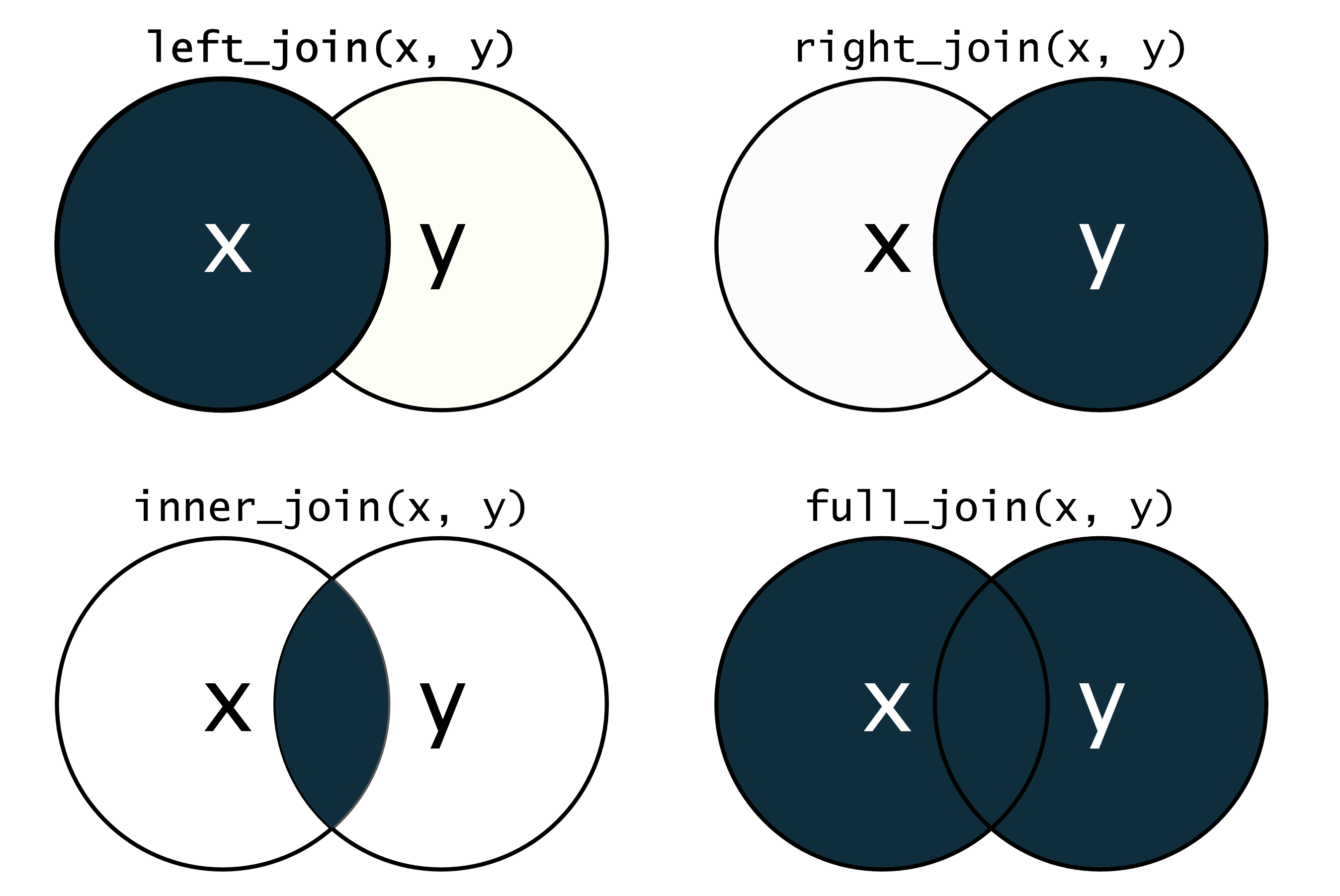
7.5 Different `*_join()` functions

8 Summary

Data transformation with dplyr

8.1 Summary I

All dplyr functions take a tibble as first argument and return a tibble.

`filter()`

pick rows with helpers
- relational and logical operators
- %in%
- is.na()
- between()
- near()

8.2 Summary II

All dplyr functions take a tibble as first argument and return a tibble.

`select()`

pick columns with helpers
- starts_with(), ends_with()
- contains()
- matches()
- any_of(), all_of()

8.3 Summary III

`arrange()`

change order of rows (adscending)
- or descending with desc()

`mutate()`

add columns but keep all columns
- case_when() for conditional values

8.4 Summary IV

`summarize()`

collapse rows into one row by some summary
- use .by argument to summarize by group

`count`

count rows based on a group

8.5 Summary V

`bind_rows()`

combine rows of multiple tibbles into one
- the tibbles need to have the same columns
- add an id column with the argument .id = "id"
- function bind_cols() works similarly just for columns

`left_join()`

combine tables based on common columns

Data handling with dplyr

1 Data transformation

1.1 Data transformation

1.2 Data transformation

1.3 Dplyr basic vocuabulary for data manipulation

1.4 Dplyr basic vocabulary

1.5 Example data

2 filter()

2.1 Useful filter() helpers

2.2 filter()

2.3 filter() + %in%

2.4 filter() + is.na()

2.5 filter() + between()

Combine different filters:

3 select()

3.1 Useful select() helpers

3.2 select()

3.3 select() + ends_with()

3.4 select() + any_of()/all_of()

3.5 select() + from:to

4 mutate()

4.1 mutate()

4.2 mutate() + case_when()

5 summarize()

5.1 summarize()

5.2 summarize() by group

5.3 count()

6 The pipe %>%

6.1 The pipe %>%

6.2 The pipe %>%

6.3 The pipe %>%

6.4 The pipe %>%

6.5 The pipe %>%

6.6 The pipe %>%