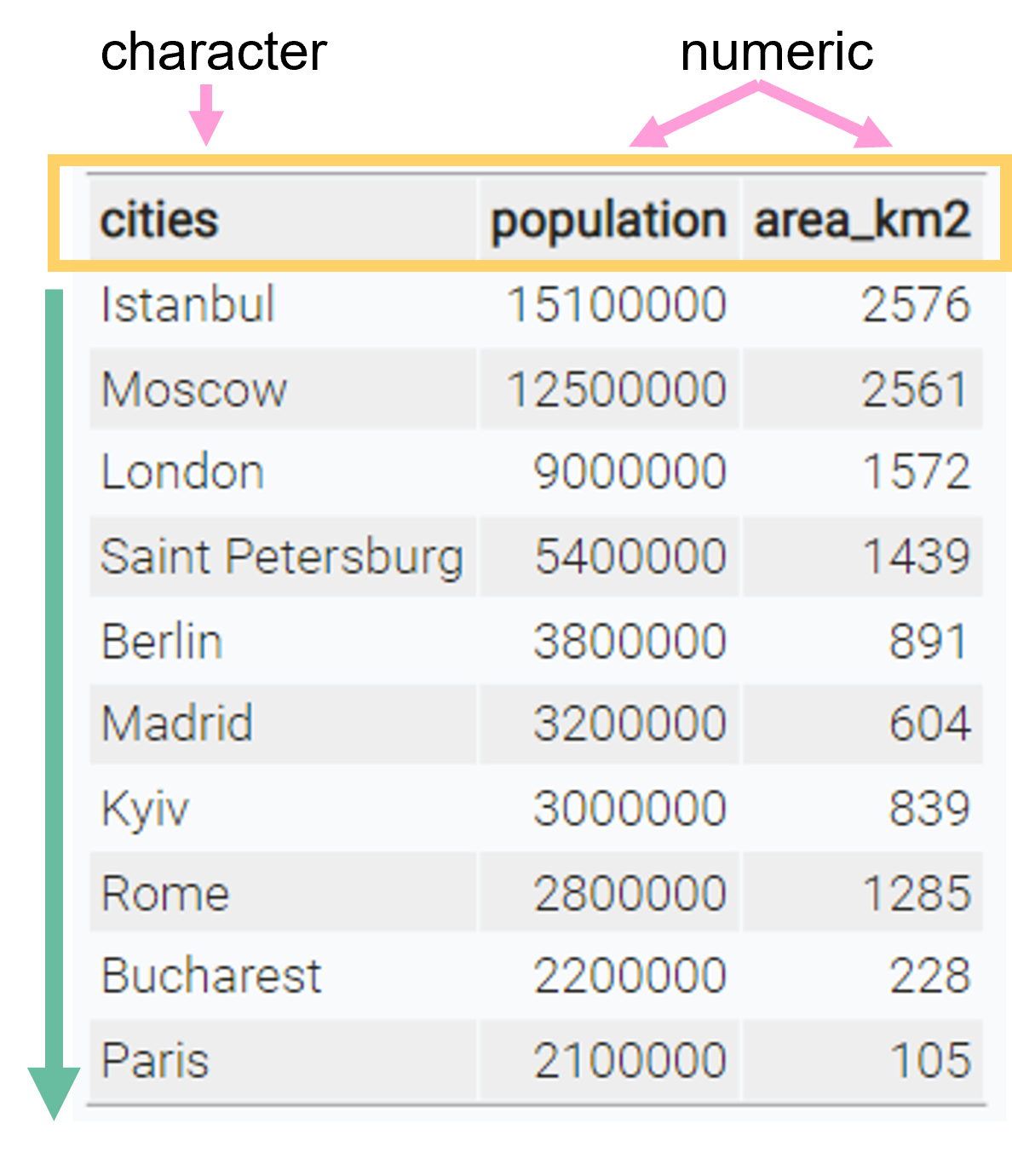
Tibbles

Day 2

Jonas Vollhüter

Freie Universität Berlin @ Theoretical Ecology

January 16, 2024

Table of contents

• 1 Data frames
• 2 Tibbles
• 3 Summary

1 Data frames

1.1 Data frames

The built-in data structure for tables in R is a data frame.

Vectors in R can’t represent data table where values are connected via rows

Data frames are one of the biggest and most important ideas in R, and one of the things that make R different from other programming languages.
(H. Wickham, Advanced R)

cities	population	area_km2
Istanbul	15100000	2576
Moscow	12500000	2561
London	9000000	1572
Saint Petersburg	5400000	1439
Berlin	3800000	891
Madrid	3200000	604
Kyiv	3000000	839
Rome	2800000	1285
Bucharest	2200000	228
Paris	2100000	105

1.2 Data frames

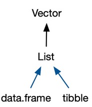
A data frame is a named list of vectors of the same length.

Basic properties of a data frame

• every column is a vector
• columns have a header
  • this is the name of the vector in the list
• within one column, all values are of the same data type
• every column has the same length

1.3 Data frames

Data frames are created with the function data.frame():

cities <- c(
  "Istanbul", "Moscow", "London", 
  "Saint Petersburg", "Berlin","Madrid",
  "Kyiv", "Rome", "Bucharest","Paris")

population <- c(
  15.1e6, 12.5e6, 9e6, 5.4e6, 3.8e6,
  3.2e6, 3e6, 2.8e6, 2.2e6, 2.1e6)

area_km2 <- c(2576, 2561, 1572, 1439, 
  891, 604, 839, 1285, 228, 105)

data.frame(
  cities = cities,
  population = population,
  area_km2 = area_km2
  )

             cities population area_km2
1          Istanbul   15100000     2576
2            Moscow   12500000     2561
3            London    9000000     1572
4  Saint Petersburg    5400000     1439
5            Berlin    3800000      891
6            Madrid    3200000      604
7              Kyiv    3000000      839
8              Rome    2800000     1285
9         Bucharest    2200000      228
10            Paris    2100000      105

2 Tibbles

Tibbles are

a modern reimagining of the data frame. Tibbles are designed to be (as much as possible) drop-in replacements for data frames.
(Wickham, Advanced R)

Have a look at this book chapter for a full list of the differences between data frames and tibbles and the advantages of using tibbles.

• Tibbles have the same basic properties as data frames (named list of vectors)

• Everything that you can do with data frames, you can do with tibbles

2.1 Tibbles

Tibbles are a available from the tibble package.

Before we use tibbles, we need to install the package once using the function install.packages:

# This has do be done only once (in the console, not in the script)
install.packages("tibble")

Then, we need to load the package into our current R session using library:

# This has to be done every time R restarts
# Put it at the top of your script
library(tibble)

2.2 Tibbles

Create a tibble using the tibble() function:

library(tibble) 

tibble(
  cities = cities,
  population = population,
  area_km2 = area_km2
)

# A tibble: 10 × 3
   cities           population area_km2
   <chr>                 <dbl>    <dbl>
 1 Istanbul           15100000     2576
 2 Moscow             12500000     2561
 3 London              9000000     1572
 4 Saint Petersburg    5400000     1439
 5 Berlin              3800000      891
 6 Madrid              3200000      604
 7 Kyiv                3000000      839
 8 Rome                2800000     1285
 9 Bucharest           2200000      228
10 Paris               2100000      105

2.4 Exploring tibbles

How many rows?

nrow(cities_tbl)

[1] 10

How many columns?

ncol(cities_tbl)

[1] 3

What are the column headers?

names(cities_tbl)

[1] "cities"     "population" "area_km2"  

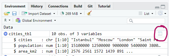
2.5 Exploring tibbles

Look at the entire table in a separate window with view():

view(cities_tbl)

Or click on the little table sign in the Environment pane:

2.6 Exploring tibbles

Get a quick summary of all columns:

summary(cities_tbl)

    cities            population          area_km2     
 Length:10          Min.   : 2100000   Min.   : 105.0  
 Class :character   1st Qu.: 2850000   1st Qu.: 662.8  
 Mode  :character   Median : 3500000   Median :1088.0  
                    Mean   : 5910000   Mean   :1210.0  
                    3rd Qu.: 8100000   3rd Qu.:1538.8  
                    Max.   :15100000   Max.   :2576.0  

2.7 Indexing tibbles

Indexing tibbles works similar to indexing vectors but with 2 dimensions instead of 1:

tibble [ row_index, col_index or col_name ]

• Missing row_index or col_index means all rows or all columns respectively.
• Indexing a tibble using [] always returns another tibble.

2.8 Indexing tibbles

# First row and first column
cities_tbl[1, 1]

# A tibble: 1 × 1
  cities  
  <chr>   
1 Istanbul

This is the same as

cities_tbl[1, "cities"]

2.9 Indexing tibbles: rows

# rows 1 & 5, all columns:
cities_tbl[c(1, 5), ]

# A tibble: 2 × 3
  cities   population area_km2
  <chr>         <dbl>    <dbl>
1 Istanbul   15100000     2576
2 Berlin      3800000      891

2.10 Indexing tibbles: columns

# All rows, first 2 columns
cities_tbl[ ,1:2] # same as cities_tbl[ , c(1, 2)]
# same as
cities_tbl[ ,c("cities", "population")]

# A tibble: 10 × 2
  cities   population
  <chr>         <dbl>
1 Istanbul   15100000
2 Moscow     12500000
3 London      9000000
# ℹ 7 more rows

2.11 Indexing tibbles: columns

Indexing columns by name is usually preferred to indexing by position

cities_tbl[ ,1:2] # okay
cities_tbl[ ,c("cities", "population")] # better

Why?

• Code is much easier to read

• Code is more robust against

  • changes in column order
  • mistakes in the code (e.g. typos)

cities_tbl[ ,c(1,3)] # 3 instead of 2 -> wrong but no error
cities_tbl[ ,c("cities", "popluation")] # typo -> wrong and error

General rule

Good code produces errors when something unintended or wrong happens

2.12 Tibbles: Select columns with $

Select an entire column from a tibble using $ (this returns a vector instead of a tibble):

cities_tbl$cities

 [1] "Istanbul"         "Moscow"           "London"           "Saint Petersburg"
 [5] "Berlin"           "Madrid"           "Kyiv"             "Rome"            
 [9] "Bucharest"        "Paris"           

2.13 Adding new columns

New columns can be added as vectors using the $ operator. The vectors need to have the same length as the tibble has rows.

# add a country column
cities_tbl$country <- c(
  "Turkey", "Russia", "UK", "Russia", "Germany", "Spain",
  "Ukraine", "Italy", "Romania", "France"
)

# A tibble: 10 × 4
   cities           population area_km2 country
   <chr>                 <dbl>    <dbl> <chr>  
 1 Istanbul           15100000     2576 Turkey 
 2 Moscow             12500000     2561 Russia 
 3 London              9000000     1572 UK     
 4 Saint Petersburg    5400000     1439 Russia 
 5 Berlin              3800000      891 Germany
 6 Madrid              3200000      604 Spain  
 7 Kyiv                3000000      839 Ukraine
 8 Rome                2800000     1285 Italy  
 9 Bucharest           2200000      228 Romania
10 Paris               2100000      105 France 

3 Summary

Tables in R: Data frames and tibbles

3.1 Summary I

data frames and tibbles

• can be used to represent tables in R
• are pretty similar, however tibbles are slightly conventient and modern
• are named lists of vectors of the same length
  • every column is a vector
  • columns have a header which is the name of the vector in the list
  • within one column, values are of same data type
  • every column has the same length

tibbles

• to use tibbles, install the package once with install.packages("tibble")
• put library(tibble) at the beginning of your script to load package

3.2 Summary II

Creating tibbles and data frames

# data frame
data.frame(
  a = 1:3,
  b = c("a", "b", "c"),
  c = c(TRUE, FALSE, FALSE) 
)
# tibble
tibble(
  a = 1:3,
  b = c("a", "b", "c"),
  c = c(TRUE, FALSE, FALSE) 
)
# convert data frame to tibble
as_tibble(df)

3.3 Summary III

Looking at tibble structure

# structure of tibble and data types of columns
str(tbl)
# number of rows
nrow(tbl)
# number of columns
ncol(tbl)
# column headers
names(tbl)
# look at the data in a new window
tibble::view(tbl)
# summary of values from each column
summary(tbl)

3.4 Summary IV

Indexing tibbles and selecting columns

Return result as tibble:

# rows and columns by position
tbl[1:3, c(1, 3)]
tbl[1:3, ] # all columns
tbl[, 3] # column 3, all rows
tbl[3] # same as above

# columns by name
tbl[, c("colA", "colB")]
tbl[c("colA", "colB")]

Return result as vector:

tbl$colA # select colA