Join relational tables
Day 3
Felix May
Freie Universität Berlin @ Theoretical Ecology
Reproduce slides
Working with several tables
- Most analysis –> data in several tables
- Need for combining or joining tables
- Mutating joins: Add new variables to one data table from matching observations in another table
- Filtering joins: filter observations from one data frame based on matching observations (or not) in another table.
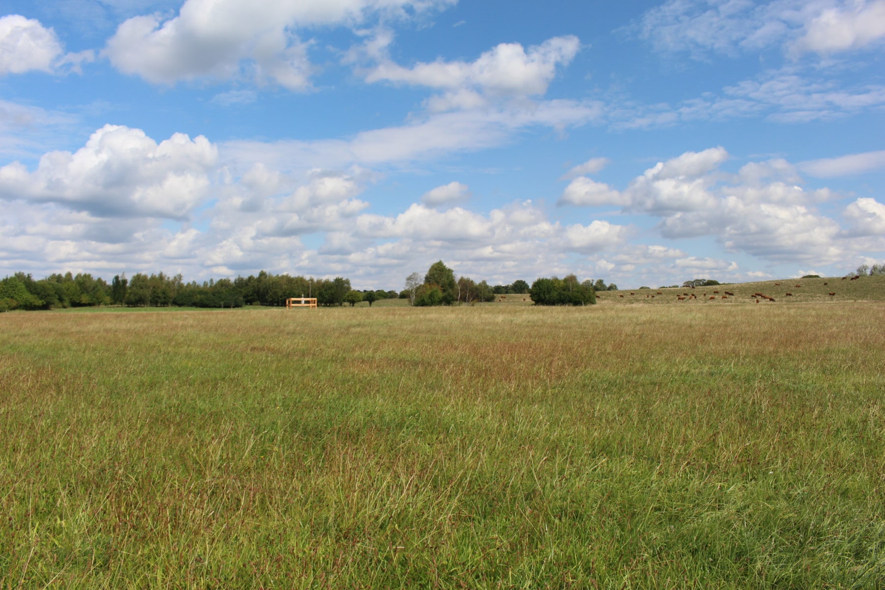
Example: Plant traits in grassland
Vegetation data from the Biodiversity Exploratories in Schorfheide-Chorin
![]()
Grassland vegetation data
- Table 1: Vegetation survey from grassland sites
vegetation <- read_csv("data/03_vegetation_schorfheide.csv")
vegetation
# A tibble: 2,196 × 4
plotID year species cover
<chr> <dbl> <chr> <dbl>
1 SEG01 2021 Carex_hirta 0.06
2 SEG01 2021 Dactylis_glomerata 0.03
3 SEG01 2021 Deschampsia_cespitosa 0.02
4 SEG01 2021 Festuca_pratensis 0.03
5 SEG01 2021 Festuca_rubra_aggr. 0.12
6 SEG01 2021 Holcus_lanatus 0.35
7 SEG01 2021 Lolium_perenne 0.001
8 SEG01 2021 Poa_pratensis_aggr. 0.005
9 SEG01 2021 Poa_trivialis 0.03
10 SEG01 2021 Potentilla_anserina 0.001
# ℹ 2,186 more rowsGrassland trait data
- Table 2: Trait values for the species
traits <- read_csv("data/03_trait_values.csv")
traits
# A tibble: 385 × 4
species SLA AMC height
<chr> <dbl> <dbl> <dbl>
1 Acer_sp NA NA NA
2 Achillea_millefolium_aggr. 0.0135 0.222 0.37
3 Acinos_arvensis NA NA 0.2
4 Aegopodium_podagraria 0.0373 0.729 0.7
5 Agrimonia_eupatoria 0.0148 0.04 0.6
6 Agrostis_capillaris 0.0294 0.358 0.23
7 Agrostis_stolonifera 0.0295 0.6 0.45
8 Ajuga_genevensis NA NA 0.19
9 Ajuga_reptans 0.0221 0.655 0.14
10 Alchemilla_vulgaris_aggr. 0.017 0.489 0.13
# ℹ 375 more rows- Trait descriptions
- SLA … Specific Leaf Area (leaf area / leaf mass)
- AMC … Arbuscular Mycorrhizal Colonisation
- height … plant height
Wanted: Mean traits for every vegetation plot –> community weighted mean traits
Joining tables – by keys
- Joining two tables: a pair of keys in both tables
- Primary key: one (or several!) variable(s) that uniquely identify each observation
- Foreign key: one (or several) variable(s) that correspond to a primary key in another table
What are the keys in this example?
- Primary key:
traits$species - Foreign key:
vegetation$species
Note
Keys do not need to have the same names in two tables, but their values have to match!
Checking primary keys
- The primary key should uniquely indentify each observation, i.e. every value should appear just once
- Check this before joining tables!
# A tibble: 385 × 2
   species                        n
   <chr>                      <int>
 1 Acer_sp                        1
 2 Achillea_millefolium_aggr.     1
 3 Acinos_arvensis                1
 4 Aegopodium_podagraria          1
 5 Agrimonia_eupatoria            1
 6 Agrostis_capillaris            1
 7 Agrostis_stolonifera           1
 8 Ajuga_genevensis               1
 9 Ajuga_reptans                  1
10 Alchemilla_vulgaris_aggr.      1
# ℹ 375 more rows
Checking primary keys
- Is there any key value with more than one occurrence?
# A tibble: 0 × 2
# ℹ 2 variables: species <chr>, n <int>- No species name appears more than once:
-
speciesis a clean primary key in this table!
Different types of joins
- Two tables
- Coulored column: key
- Grey column: values
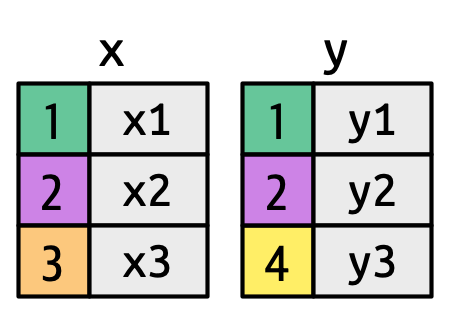
- Different joins function in
dplyrpackageinner_joinleft_joinright_joinfull_join
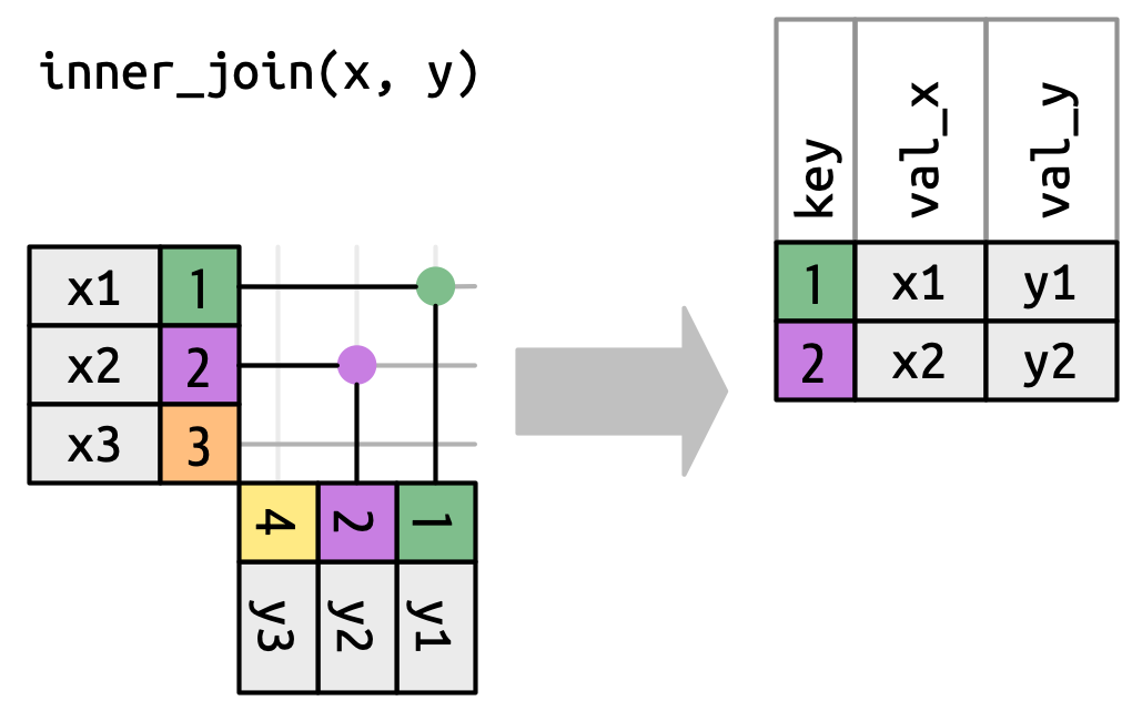
Which lines will be in the joined table?
Inner join
- Keep only rows with matching keys in both tables
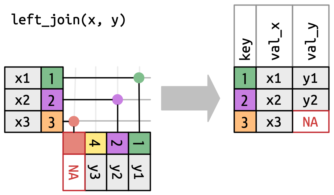
Left join
- Keep all the rows of Table x (Table 1)
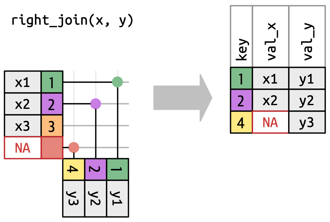
Right join
- Keep all the rows of Table y (Table 2)
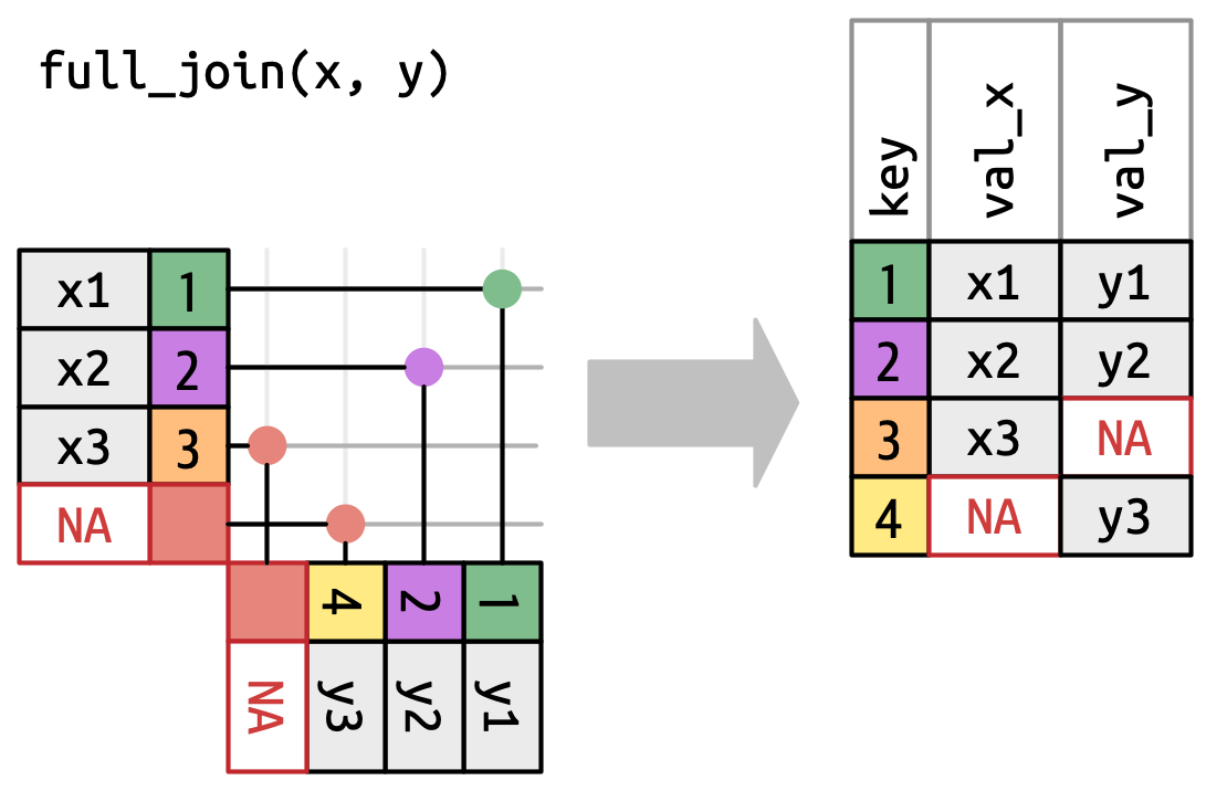
Full join
- Keep all rows of Tables x and y (Tables 1 + 2)
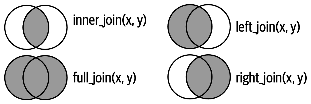
Joins as Venn diagrams
Join vegetation and traits
- Add trait values to vegetation data –> left join
veg_traits <- left_join(vegetation, traits)
veg_traits <- vegetation %>% left_join(traits)
veg_traits
# A tibble: 2,196 × 7
plotID year species cover SLA AMC height
<chr> <dbl> <chr> <dbl> <dbl> <dbl> <dbl>
1 SEG01 2021 Carex_hirta 0.06 0.019 0.162 0.38
2 SEG01 2021 Dactylis_glomerata 0.03 0.0241 0.072 0.41
3 SEG01 2021 Deschampsia_cespitosa 0.02 0.0126 0.409 0.28
4 SEG01 2021 Festuca_pratensis 0.03 0.0213 0.203 0.4
5 SEG01 2021 Festuca_rubra_aggr. 0.12 0.0199 0.187 0.3
6 SEG01 2021 Holcus_lanatus 0.35 0.0279 0.053 0.43
7 SEG01 2021 Lolium_perenne 0.001 0.0219 0.546 0.25
8 SEG01 2021 Poa_pratensis_aggr. 0.005 0.0237 NA 0.29
9 SEG01 2021 Poa_trivialis 0.03 0.0326 NA 0.39
10 SEG01 2021 Potentilla_anserina 0.001 0.0186 NA 0.09
# ℹ 2,186 more rowsCalculate community mean traits
- Community mean traits
- Unweighted –> Equal weight of every species
- Weighted –> use
coveras weight when calculating the mean traits
# A tibble: 99 × 4
# Groups:   plotID [50]
   plotID  year   mSLA mSLA_w
   <chr>  <dbl>  <dbl>  <dbl>
 1 SEG01   2021 0.0224 0.0248
 2 SEG01   2022 0.0226 0.0176
 3 SEG02   2021 0.0238 0.0253
 4 SEG02   2022 0.0216 0.0231
 5 SEG03   2021 0.0249 0.0232
 6 SEG03   2022 0.0229 0.0223
 7 SEG04   2021 0.0222 0.0226
 8 SEG04   2022 0.0220 0.0232
 9 SEG05   2021 0.0239 0.0260
10 SEG05   2022 0.0234 0.0279
# ℹ 89 more rows
Complete analysis in one step
community_traits <- vegetation %>%
  left_join(traits) %>%
  group_by(plotID, year) %>%
  summarise(
    mSLA   = mean(SLA, na.rm = T),
    mSLA_w = weighted.mean(SLA, cover, na.rm = T),
    mheight   = mean(height, na.rm = T),
    mheight_w = weighted.mean(height, cover, na.rm = T),
  )
community_traits
# A tibble: 99 × 6
# Groups: plotID [50]
plotID year mSLA mSLA_w mheight mheight_w
<chr> <dbl> <dbl> <dbl> <dbl> <dbl>
1 SEG01 2021 0.0224 0.0248 0.307 0.390
2 SEG01 2022 0.0226 0.0176 0.36 0.320
3 SEG02 2021 0.0238 0.0253 0.372 0.387
4 SEG02 2022 0.0216 0.0231 0.428 0.432
5 SEG03 2021 0.0249 0.0232 0.389 0.547
6 SEG03 2022 0.0229 0.0223 0.527 0.595
7 SEG04 2021 0.0222 0.0226 0.841 0.54
8 SEG04 2022 0.0220 0.0232 0.573 0.556
9 SEG05 2021 0.0239 0.0260 0.443 0.483
10 SEG05 2022 0.0234 0.0279 0.484 0.460
# ℹ 89 more rowsExercise
Now it is your turn!
Join relational tables