Statistic - Basics
Day 4
Freie Universität Berlin @ Theoretical Ecology
January 18, 2024
Pleas note: An AI tool was used to create the following content (ChatGPT, 2024).
1 Descriptive vs. Exploratory Statistics
Descriptive Statistics
- Goal: Describe and summarize data.
- Focus: Providing a summary of key features in a dataset.
- Methods:
- Measures of central tendency (mean, median, mode).
- Measures of dispersion (range, variance, standard deviation).
- Visualization techniques (histograms, box plots).
Exploratory Statistics
- Goal: Discover patterns, relationships, or trends in data.
- Focus: Generating hypotheses and uncovering hidden structures.
- Methods:
- Data exploration through visualizations.
- Hypothesis generation without predefined expectations.
- Flexible analysis to adapt to new discoveries.
Key Differences
- Descriptive Statistics:
- Summarizes existing data.
- Focuses on numerical and graphical summaries.
- Often used for reporting and presentation.
- Exploratory Statistics:
- Explores new insights in data.
- Emphasizes hypothesis generation.
- Allows for flexibility and adaptability in analysis.
When to Use Each?
- Descriptive Statistics:
- Initial understanding of data.
- Reporting key features.
- Exploratory Statistics:
- Seeking new patterns or relationships.
- Generating hypotheses for further testing.
Conclusion
- Both types of statistics play crucial roles in data analysis.
- Descriptive statistics provide a foundation for understanding data.
- Exploratory statistics help uncover hidden insights and guide further research.
2 Statistical parameters
Arithmetic mean
Definition:
- The arithmetic mean, also known as the average, is a measure of central tendency that represents the sum of all values in a dataset divided by the number of values.
Formula: \[ \bar{X} = \frac{1}{n} \sum_{i=1}^{n} x_i \]
Key Points:
- Provides a representative value for the central position of the data.
- Sensitive to extreme values (outliers) in the dataset.
- Calculated by adding up all values and dividing by the number of values.
- Use Cases:
- Commonly used in statistics to summarize data.
- Provides a single, numerical summary of the dataset.
- Example:
- If we have values {4, 6, 8, 10} the arithmetic mean would be \[ \frac{1}{4} \cdot (4 + 6 + 8 + 10) = 7 \]
- Considerations:
- May not accurately represent the data if there are extreme values.
- Useful for understanding the central tendency of a dataset.
3 Median
- median: numerical value separating the higher half of a data sample from the lower half
- n odd:
- sort the data by its size -> median is right in the middle
- example: x1= 5, x2= 2, x3= -3, x4= 7, x5= 4
- order: -3, 2, 4, 5, 7
- -> median = 4
- n even:
- mean value of the two middle values
- example: x1= 5, x2= 2, x3= -3, x4= 7, x5= 4, x6= 1 order: -3, 1, 2, 4, 5, 7 -> median = (2+4)/2 = 3
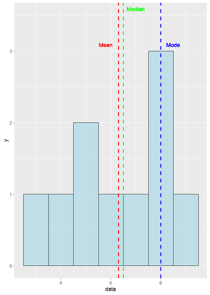
Example
Data: {3, 4, 5, 5, 6, 7, 8, 8, 8, 9}
4 Mode
Definition
Mode is a statistical measure that represents the most frequently occurring value (or values) in a dataset. Unlike mean and median, the mode is concerned with the frequency of values rather than their central tendency.
Types of Mode
- Unimodal:
- A dataset has one mode if it has only one value with the highest frequency.
- Bimodal:
- A dataset has two modes if it has two values with equal highest frequencies.
- Multimodal:
- A dataset has more than two modes if it has multiple values with the highest frequencies.
Calculating Mode
For discrete data, the mode is simply the value with the highest frequency.
For continuous data, the mode is often identified graphically or through statistical software.
5 Variance
- Relate sum of squares to number of data points -> divide by (n-1)
- why (n-1) and not n?
- only (n-1) allows for an unbiased estimation (erwartungstreu) of the true variance
- number of data points corrected by -1, since one degree of freedom was lost when estimating the mean (which is used to calculate the variance)
\[ \begin{align} s^2 = \frac{\sum_{i=1}^n \left( x_i - \overline{x}\right)^2}{n - 1} \end{align} \]
6 Standard deviation
\[ \begin{align} s = \sqrt{s^2} = \sqrt{\frac{\sum_{i=1}^n \left(x_i - \overline{x} \right)^2}{n - 1}} \end{align} \]
Definition
Standard Deviation is a measure of the amount of variation or dispersion in a set of values. It quantifies how much individual data points differ from the mean (average) of the data set.
Interpretation
- A low standard deviation indicates that the data points are close to the mean, suggesting less variability.
- A high standard deviation suggests that the data points are spread out over a wider range, indicating greater variability.
7 Standard Error of the Mean (SEM)
Definition
Standard Error of the Mean (SEM) is a measure of how much the sample mean is expected to vary from the true population mean. It quantifies the precision or reliability of the sample mean as an estimate of the population mean.
Formula
The formula for calculating SEM is:
\[ \begin{align} sem = \frac{s}{\sqrt{n}} \end{align} \]
- s is the sample standard deviation.
- N is the sample size.
Characteristics
A smaller SEM indicates a more precise estimate of the population mean.
A larger SEM suggests greater variability in the sample mean and less precision.
SEM is often used to calculate confidence intervals around the sample mean. The wider the confidence interval, the less precise the estimate of the population mean.
8 Residuals: Sum of square error
\[ \begin{align} \sum_{i=1}^{n}\left(x_i - \overline{x}\right)^2 \end{align} \]
Introduction to R