Statistical tests

Day 5

Jonas Vollhüter & Felix Nößler

Freie Universität Berlin @ Theoretical Ecology

January 19, 2024

Reproduce slides

library(dplyr)
library(tidyr)
library(ggplot2)

## theme for ggplot
theme_set(theme_classic())
theme_update(text = element_text(size = 14))

1 Introduction to null-hypothesis significance testing

procedure:

formulate a null hypothesis (\(H_0\)) and an alternative hypothesis (\(H_1\))
collect data
calculate the probability of observing data at least as extreme if \(H_0\) was true (p-value)
if p-value < \(\alpha\): reject \(H_0\) (typically \(\alpha = 0.05\))

2 P-values

is used in null-hypothesis significance testing
is the probability of obtaining test results at least as extreme as the result actually observed, under the assumption that the null hypothesis is correct

Please note the discussion going on about p-values as a basis for binary decisions. See e.g. here or here as a starting point

Which factors influence the p-value?

Variability in the data
Effect size
Sample size

please report all of them in your report/article

3 Simulation study on p-values

Life expectancy

simulate life expectancy of 100 people with a log-normal distribution
we then compare the life expectancy of two groups (control, treatment) with a Wilcoxon test

x <- rlnorm(100, meanlog = log(75), sdlog = 0.12)

ggplot() +
  geom_histogram(aes(x), breaks = seq(50, 120, 2))

No difference in life expectancy

p_values <- c()
for (i in 1:2000) {
  x_control <- rlnorm(100, meanlog = log(75), sdlog = 0.12)
  x_treatment <- rlnorm(100, meanlog = log(75), sdlog = 0.12)
  p_val <- wilcox.test(x_control, x_treatment)$p.value
  p_values <- c(p_values, p_val)
}

mean(p_values < 0.05)

[1] 0.051

Code

plotting_df <- tibble(p_values = p_values,
                      color = ifelse(p_values < 0.05, "significant", "non-significant"))
ggplot(plotting_df) +
  geom_histogram(aes(p_values, fill = color), bins = 100,
                 breaks = seq(0, 1, 0.05)) +
  scale_fill_manual(values = c("significant" = "red", "non-significant" = "grey")) +
  labs(fill = "", x = "p-value")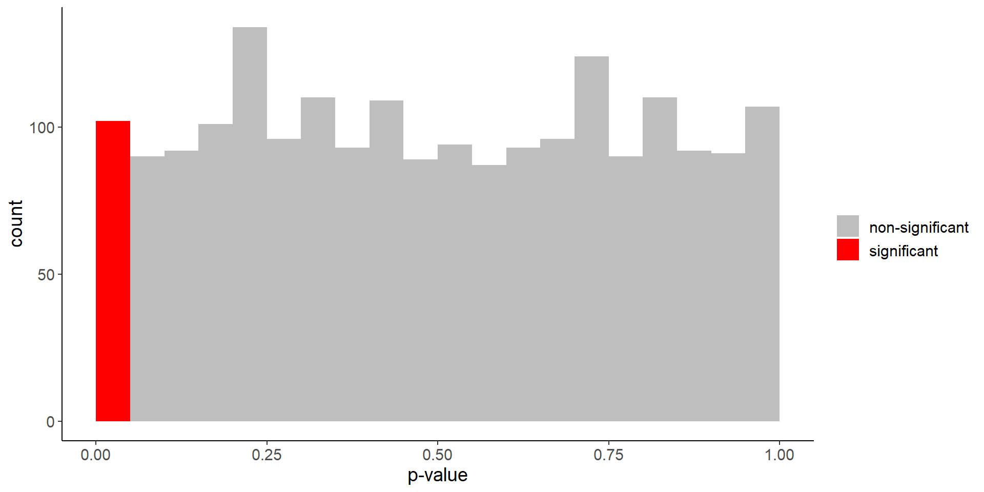

Difference in life expectancy

p_values <- c()
for (i in 1:2000) {
  x_control <- rlnorm(100, meanlog = log(75), sdlog = 0.12)
  x_treatment <- rlnorm(100, meanlog = log(77), sdlog = 0.12)
  p_val <- wilcox.test(x_control, x_treatment)$p.value
  p_values <- c(p_values, p_val)
}

mean(p_values < 0.05)

[1] 0.317

Code

plotting_df <- tibble(p_values = p_values,
                      color = ifelse(p_values < 0.05, "significant", "non-significant"))
ggplot(plotting_df) +
  geom_histogram(aes(p_values, fill = color), bins = 100,
                 breaks = seq(0, 1, 0.05)) +
  scale_fill_manual(values = c("significant" = "red", "non-significant" = "grey")) +
  labs(fill = "", x = "p-value")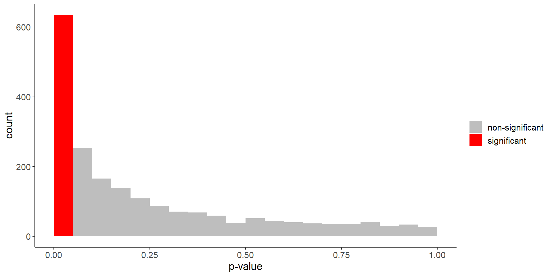

Difference in life expectancy

p_values <- c()
for (i in 1:2000) {
  x_control <- rlnorm(10, meanlog = log(75), sdlog = 0.12)
  x_treatment <- rlnorm(10, meanlog = log(77), sdlog = 0.12)
  p_val <- wilcox.test(x_control, x_treatment)$p.value
  p_values <- c(p_values, p_val)
}

mean(p_values < 0.05)

[1] 0.061

Code

plotting_df <- tibble(p_values = p_values,
                      color = ifelse(p_values < 0.05, "significant", "non-significant"))
ggplot(plotting_df) +
  geom_histogram(aes(p_values, fill = color), bins = 100,
                 breaks = seq(0, 1, 0.05)) +
  scale_fill_manual(values = c("significant" = "red", "non-significant" = "grey")) +
  labs(fill = "", x = "p-value")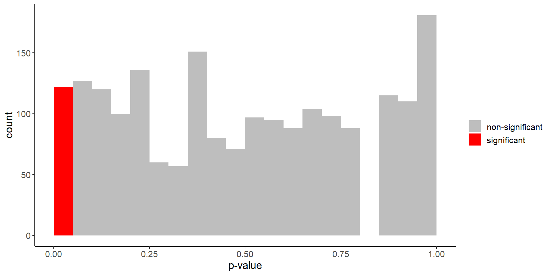

Difference in life expectancy

p_values <- c()
for (i in 1:2000) {
  x_control <- rlnorm(100, meanlog = log(75), sdlog = 0.12)
  x_treatment <- rlnorm(100, meanlog = log(80), sdlog = 0.12)
  p_val <- wilcox.test(x_control, x_treatment)$p.value
  p_values <- c(p_values, p_val)
}

mean(p_values < 0.05)

[1] 0.9595

Code

plotting_df <- tibble(p_values = p_values,
                      color = ifelse(p_values < 0.05, "significant", "non-significant"))
ggplot(plotting_df) +
  geom_histogram(aes(p_values, fill = color), bins = 100,
                 breaks = seq(0, 1, 0.05)) +
  scale_fill_manual(values = c("significant" = "red", "non-significant" = "grey")) +
  labs(fill = "", x = "p-value")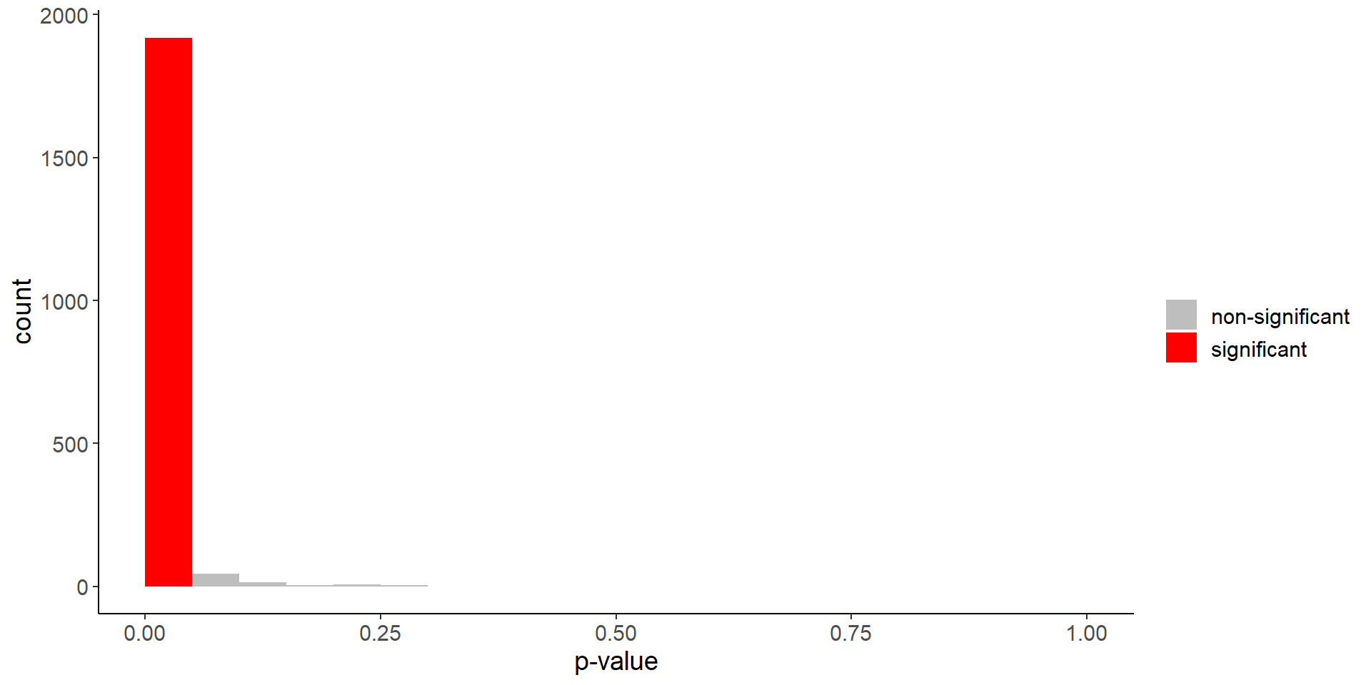

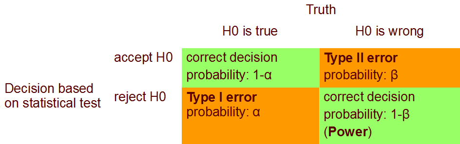
4 Errors in statistical tests

5 Pitfalls - thinks to keep in mind

statistical significance does not imply biological significance
the null hypothesis is almost never true
no statistical significance does not imply no effect
arbitrary choice of \(\alpha\) (typically 0.05)

see e.g. here

Please dont’t do:

p-hacking: trying out different tests until you find a significant result
data dredging: trying out different subsets of your data until you find a significant result
multiple testing: doing multiple tests on the same data until you find a significant result (without correcting for multiple testing)

6 Test for equal means (distribution)

t-test

Normal distribution AND equal variance
Compares if mean values are within range of standard error of each other
p: how likely is the difference if the means were equal

Welch-Test

Normal distribution but unequal variance
Corrected t-test

Wilcoxon rank sum test (Mann–Whitney U test)

Non-normal distribution and unequal variance
Compares rank sums of the data
Non-parametric

Example dataset

InsectSprays: counts of insects in agricultural experimental units treated with different insecticides

TreatA <- filter(
  InsectSprays,
  spray == "A")$count
TreatB <- filter(
  InsectSprays,
  spray == "B")$count
TreatC <- filter(
  InsectSprays,
  spray == "C")$count

t-test

\(H_0\): The samples do not differ in their mean

Treatment A and B: normally distributed and equal variance

t.test(TreatA, TreatB, var.equal = TRUE)


    Two Sample t-test

data:  TreatA and TreatB
t = -0.45352, df = 22, p-value = 0.6546
alternative hypothesis: true difference in means is not equal to 0
95 percent confidence interval:
 -4.643994  2.977327
sample estimates:
mean of x mean of y 
 14.50000  15.33333

t: test statistics (t = 0 means equal means)
df: degrees of freedom of t-statistics
p-value: how likely is it to observe the data if \(H_0\) was true?

t-test

\(H_0\): The samples do not differ in their mean

Treatment A and B: normally distributed and equal variance

t.test(TreatA, TreatB, var.equal = TRUE)


    Two Sample t-test

data:  TreatA and TreatB
t = -0.45352, df = 22, p-value = 0.6546
alternative hypothesis: true difference in means is not equal to 0
95 percent confidence interval:
 -4.643994  2.977327
sample estimates:
mean of x mean of y 
 14.50000  15.33333

Result: The means of spray A and B don’t differ significantly (t = -0.45, df = 22, p = 0.66)

Welch-Test

\(H_0\): The samples do not differ in their mean

Treatment A and C: normally distributed and non-equal variance

t.test(TreatA, TreatC, var.equal = FALSE)


    Welch Two Sample t-test

data:  TreatA and TreatC
t = 8.4073, df = 14.739, p-value = 5.278e-07
alternative hypothesis: true difference in means is not equal to 0
95 percent confidence interval:
  9.263901 15.569433
sample estimates:
mean of x mean of y 
14.500000  2.083333

Result: The means of spray A and C do differ significantly (t = 7.58, df = 13.9, p < 0.001)

Wilcoxon-rank-sum Test (Mann–Whitney U test)

\(H_0\): For randomly selected values X and Y from two populations, the probability of X being greater than Y is equal to the probability of Y being greater than X (if both populations have a similar type of distribution and variance: both medians are equal).

wilcox.test(TreatA, TreatB)


    Wilcoxon rank sum test with continuity correction

data:  TreatA and TreatB
W = 62, p-value = 0.5812
alternative hypothesis: true location shift is not equal to 0

Result: We cannot reject the null hypothesis that the probability of counted insects from treatment A being greater than the counted insects from treatment B is equal to the probability of the counted insects from treatment B being greater than the counted insects from treatment A (W = 62, p = 0.58).

Paired values

Are there pairs of data points?

Example: samples of invertebrates across various rivers before and after sewage plants.

For each plant, there is a pair of data points (before and after the plant)
Question: Is the change (before-after) significant

Use paired = TRUE in the test.

t.test(TreatA, TreatB, var.equal = TRUE, paired = TRUE)
t.test(TreatA, TreatB, var.equal = FALSE, paired = TRUE)
wilcox.test(TreatA, TreatB, paired = TRUE)

Careful: your treatment vector both have to have the same order

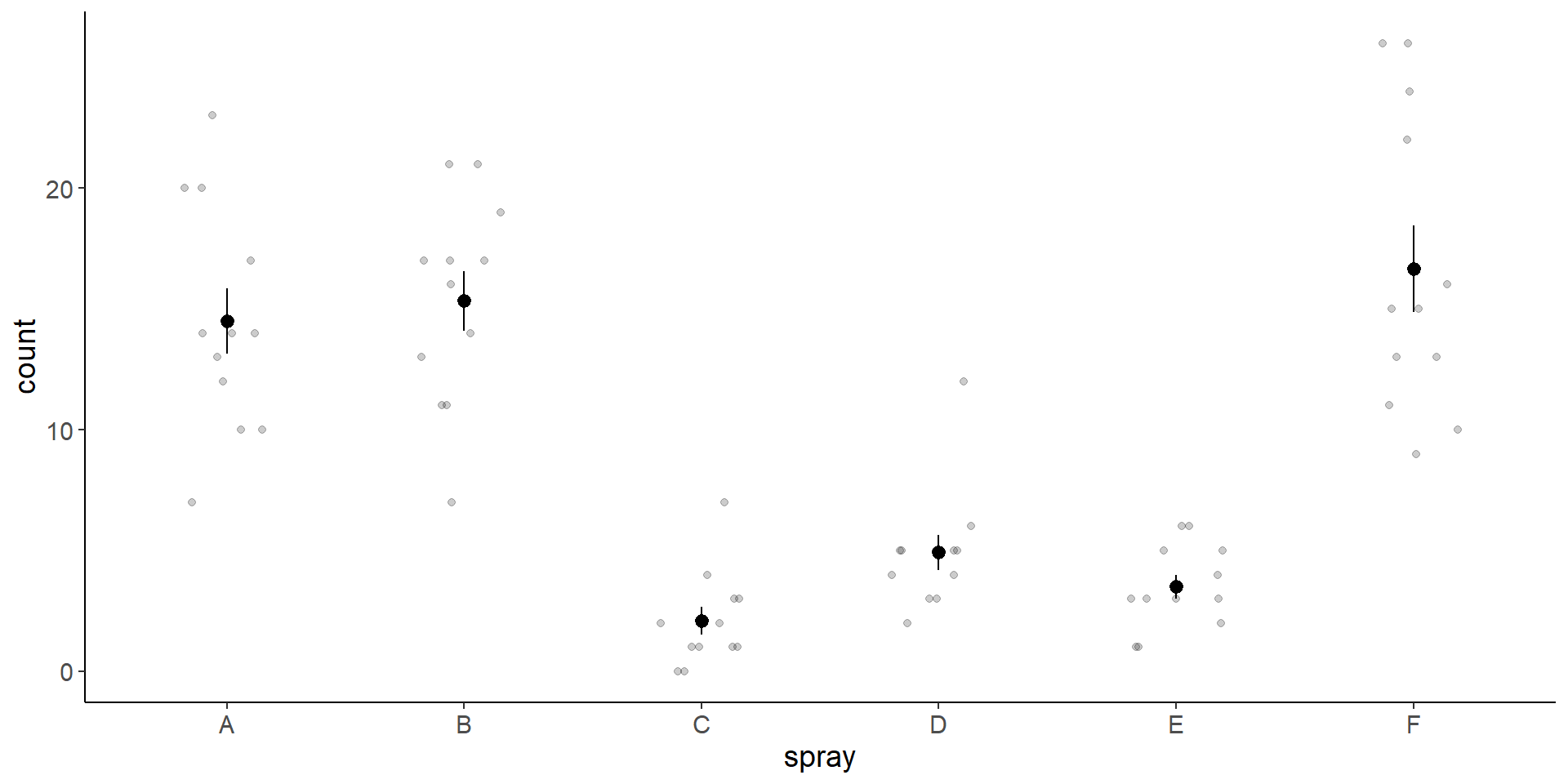
Note: Plot mean +- se using `stat_summary`

One way to plot the results is to plot mean and standard error of the mean:

ggplot(InsectSprays, aes(x = spray, y = count)) +
  geom_jitter(width = 0.2, height = 0, alpha = 0.2) +
  stat_summary(fun.data = mean_se)

Statistical tests

Reproduce slides

1 Introduction to null-hypothesis significance testing

2 P-values

Which factors influence the p-value?

3 Simulation study on p-values

Life expectancy

No difference in life expectancy

Difference in life expectancy

Difference in life expectancy

Difference in life expectancy

4 Errors in statistical tests

5 Pitfalls - thinks to keep in mind

6 Test for equal means (distribution)

Example dataset

t-test

t-test

Welch-Test

Wilcoxon-rank-sum Test (Mann–Whitney U test)

Paired values

Note: Plot mean +- se using stat_summary

Note: Plot mean +- se using `stat_summary`