Probability and Likelihood
Day 4
January 18, 2024
3 Probability
- How would you quantify the probability that someone in this room is taller than 175 cm if we pick someone randomly? Imagine 16 are smaller and 4 are taller than 175 cm.
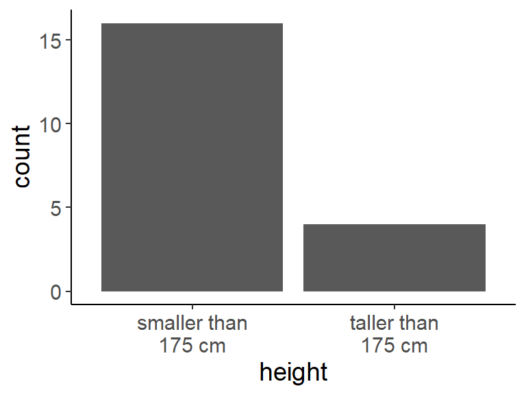
- Solution: \(\frac{4}{16+4} = 0.2\)
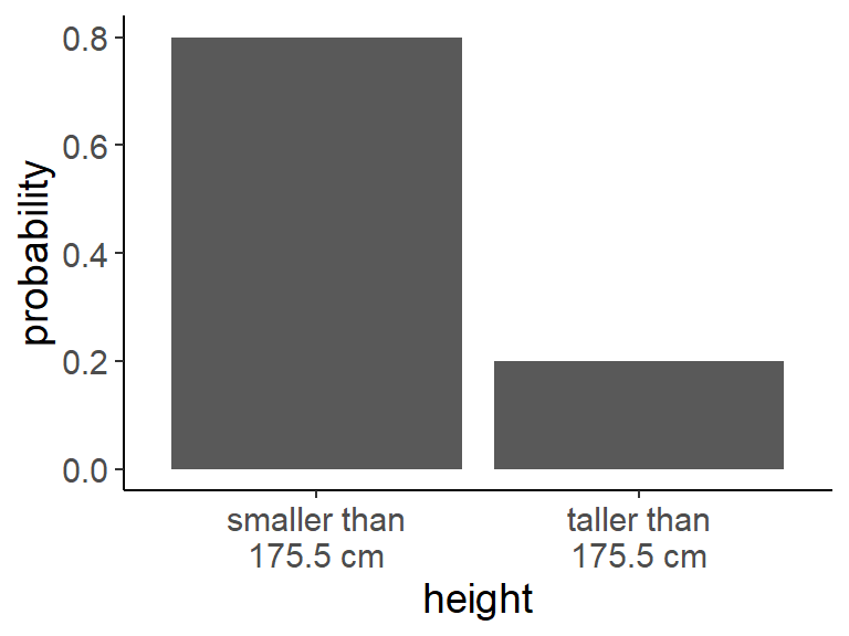
4 Probability mass functions
- out of this example, we can constuct the probability mass function (pmf)
- the pmf is a function that gives the probability that a discrete random variable is exactly equal to some value
- the probabilties of all possible outcomes sum up to 1
5 Probability
- How would you quantify the probability that someone in this room is taller than 175 cm and smaller than 180 cm?
Code
heights <- c(162.5991, 169.7083, 154.8859, 176.9837, 152.9955,
             166.7666, 170.8611, 156.8119, 152.9782, 181.7327,
             166.3193, 162.3588, 163.0147, 175.8846, 164.3344,
             171.851, 169.1128, 165.527, 179.5642, 157.6616)

ggplot() +
  geom_histogram(aes(heights), breaks = seq(140, 195, 5)) +
  annotate("rect", xmin = 175, xmax = 180, ymin = 0, ymax = 3,
           fill = "blue", alpha = 0.7) +
  scale_x_continuous(breaks = seq(140, 195, 5))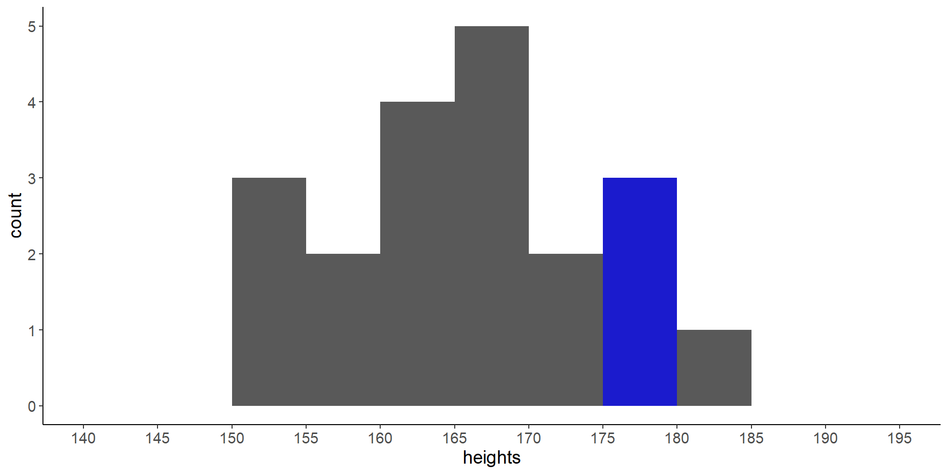
- the solution: \(\frac{3}{20} = 0.15\)
6 Probability mass function
- we can construct a probability mass function (pmf) and cumulative distribution function (cdf) for the discrete random variable
Code
df <- tibble(
  height = seq(142.5, 192.5, 5.0),
  count = as.numeric(
    table(cut(heights, breaks = seq.int(from = 140, to = 195, by = 5)))),
  pmf = count / sum(count),
  cdf = cumsum(pmf)) %>%
  select(-count) %>%
  pivot_longer(c(pmf, cdf), names_to = "group", values_to = "y") %>%
  mutate(y = y + 0.001,
         group = factor(group, levels = c("pmf", "cdf")))

ggplot(aes(x = height, y = y), data = df) +
  geom_col() +
  scale_x_continuous(breaks = seq(140, 195, 5)) +
  labs(y = "probability") +
  facet_grid(group ~ .) +
  theme_light() +
  theme(text = element_text(size = 14))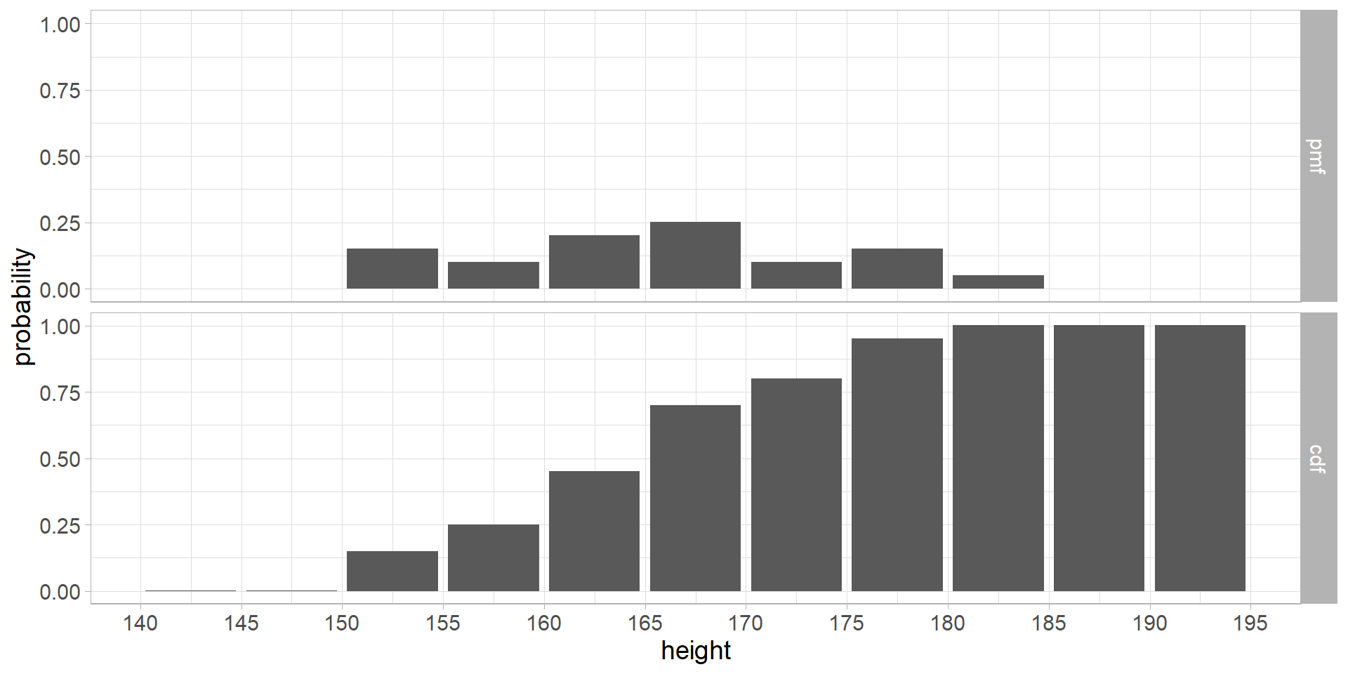
8 Let’s use a continous distribution
Code
lm1 <- lm(heights ~ 1)
sd1 <- sigma(lm1) # equivalent to sd(heights)
m1 <- coef(lm1)   # equivalent to mean(heights)

df <- tibble(
  height = seq(142.5, 192.5, 5.0),
  count = as.numeric(
    table(cut(heights, breaks = seq.int(from = 140, to = 195, by = 5)))),
  density = count / sum(count))

df_norm <- tibble(
  height = seq(140, 195, length.out = 200),
  density = dnorm(height, mean = m1, sd = sd1))

ggplot() +
  geom_col(aes(y = density, x = height), width = 4.8, data = df) +
  geom_point(aes(x = height, y = 0.008), data = tibble(height = heights),
              size = 4,
               alpha = 0.6, color = "blue",
             position = position_jitter(seed = 2, width = 0, height = 0.008)) +
  geom_line(aes(x = height, y = density), data = df_norm, linewidth = 2, color = "red") +

  scale_x_continuous(breaks = seq(140, 195, 5)) +
  labs(y = "density / probability")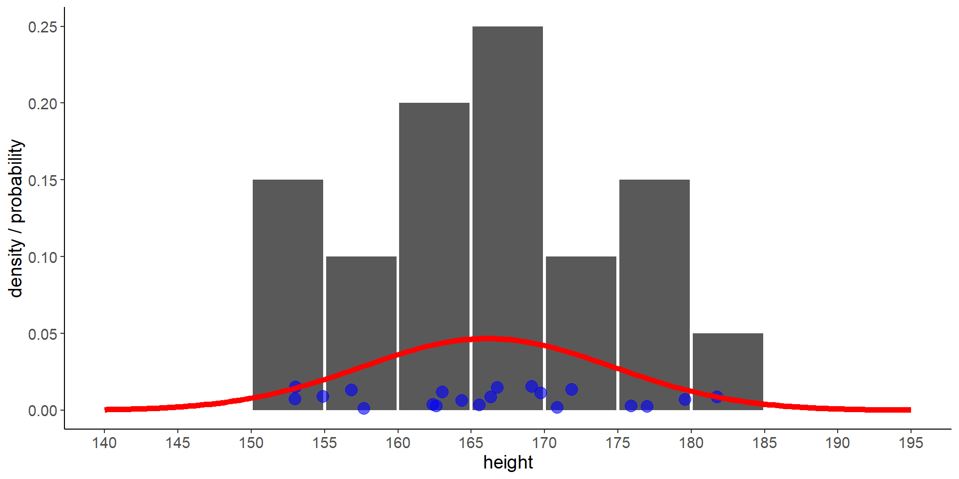
9 Probability for continous distributions
- what is the probability that a person is between 185 cm and 190 cm tall?
- in contrast to discrete distributions, we have to calculate the area under the curve of the probability density function (pdf) to get the probability
Code
ggplot() +
  geom_ribbon(aes(x = height, ymin = 0, ymax = density),
              data = filter(df_norm, height >= 185 & height <= 190),
            fill = "purple", alpha = 0.5) +
  geom_line(aes(x = height, y = density), data = df_norm,
            color = "red", linewidth = 2) +
  scale_x_continuous(breaks = seq(140, 195, 5))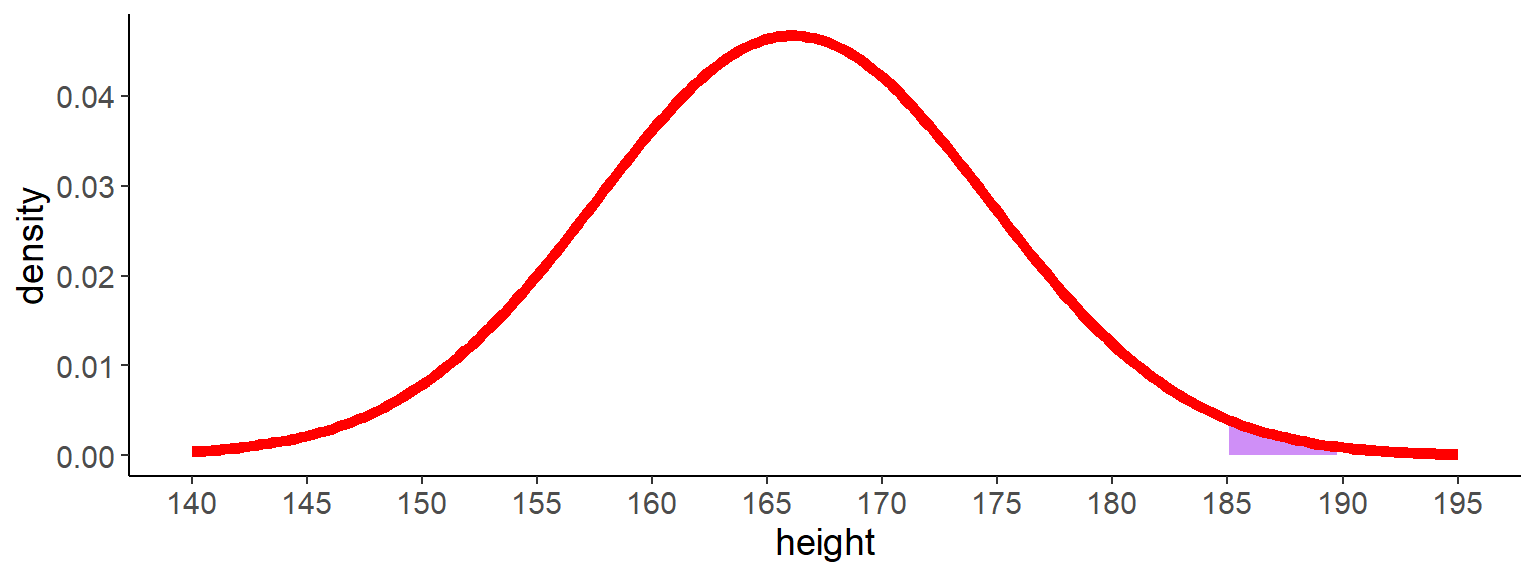
Note
Probability density functions are used for continous distributions, probability mass functions for discrete distributions.
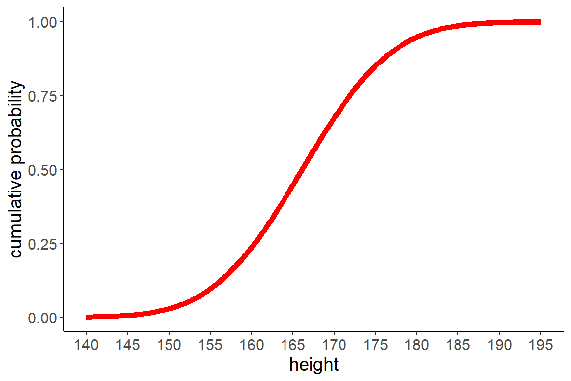
10 Cumulative distribution function
- the cumulative distribution function (cdf) for a continous distribution sums up the probability of all values smaller than a given value \(x\)
- the cdf is the integral (sums up the area under the curve) of the pdf
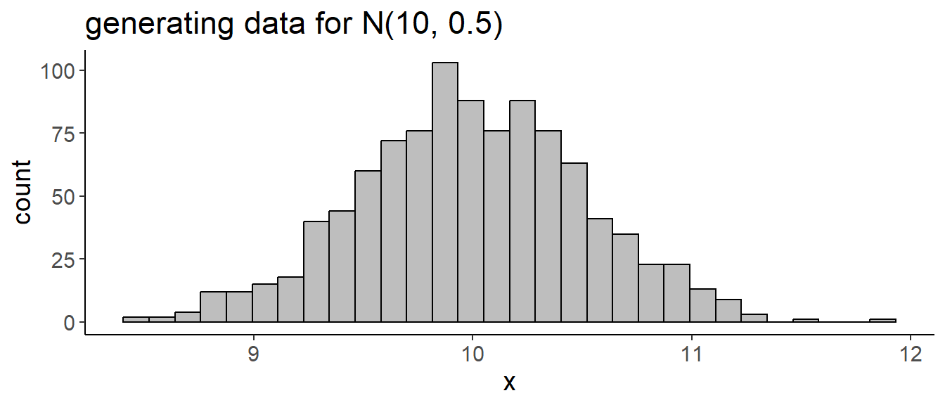
13 What else can we do with a (Normal) distribution
Tip: Distribution zoo
the distribution zoo is a great tool to explore different distributions and what you can do with them
we can generate random numbers from a fitted distribution:
we can ask how tall a person is that is the 70 % percentile of the population:
- we use the inverse cumulative distribution function (quantile function) to calculate this:
qnorm(0.7, mean = 166, sd = 8)[1] 170.195214 But how do we fit a distribution to data?
let’s start with fitting the mean \(\mu\) to the data:
Code
df <- tibble(height = heights)

some_distributions <- tibble(
  height = seq(140, 195, length.out = 200),
  `150` = dnorm(height, mean = 150, sd = 10),
  `166` = dnorm(height, mean = 166, sd = 10),
  `180` = dnorm(height, mean = 180, sd = 10)) %>%
  pivot_longer(-height, names_to = "name", values_to = "y")

ggplot() +
  geom_point(aes(x = height, y = 0.001), data = df,
              size = 4,
               alpha = 0.6, color = "blue",
             position = position_jitter(seed = 2, width = 0, height = 0.001)) +
  geom_line(aes(x = height, y = y, color = name), data = some_distributions,
            linewidth = 2) +
  labs(y = "density",
       title = "Which distribution fits the data best?",
       color = "Mean")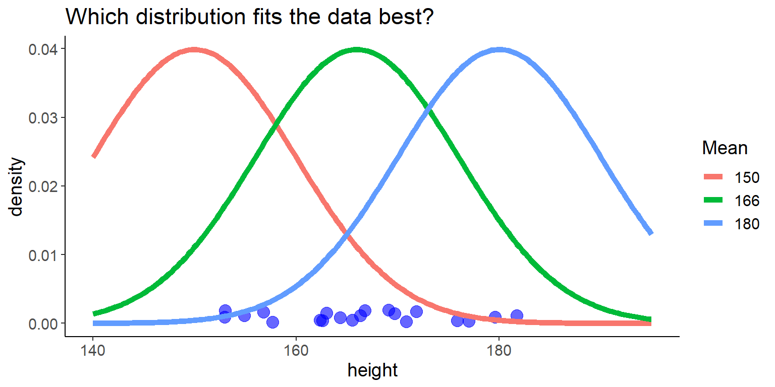
now, we fit the standard deviation \(\sigma\):
Code
some_distributions <- tibble(
  height = seq(140, 195, length.out = 200),
  `2` = dnorm(height, mean = 166, sd = 2),
  `10` = dnorm(height, mean = 166, sd = 10),
  `20` = dnorm(height, mean = 166, sd = 20)) %>%
  pivot_longer(-height, names_to = "name", values_to = "y") %>%
  mutate(name = fct_reorder(name, as.numeric(name)))

ggplot() +
  geom_point(aes(x = height, y = 0.001), data = df,
              size = 4,
               alpha = 0.6, color = "blue",
             position = position_jitter(seed = 2, width = 0, height = 0.001)) +
  geom_line(aes(x = height, y = y, color = name), data = some_distributions,
            linewidth = 2) +
  labs(y = "density",
       title = "Which distribution fits the data best?",
       color = "Standard\n deviation")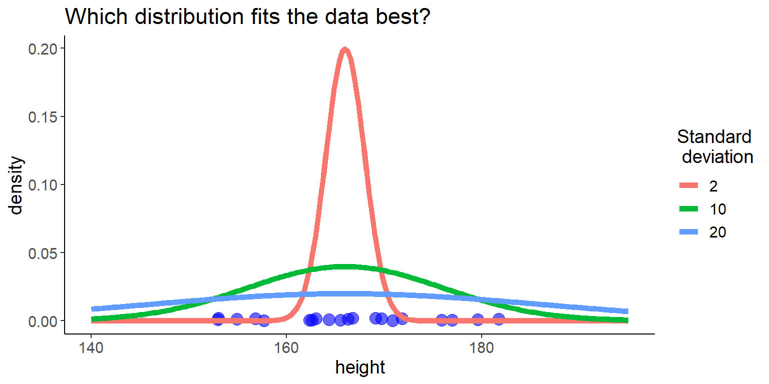
16 Likelihood visualization
- we calculate the likelihood given our data for \(\mathcal{N}(\mu = 170,\,\sigma = 10)\)
Code
df <- tibble(height = heights)
mu <- 170
sigma <- 10

likelihood_df <- tibble(
  height = heights,
  density = dnorm(height, mean = mu, sd = sigma))

dens_df <- tibble(
  height = seq(140, 195, length.out = 200),
  density = dnorm(height, mean = mu, sd = sigma))

ggplot(aes(x = height, y = 0), data = df) +
  geom_line(aes(y = density), data = dens_df,
            color = "red", linewidth = 2) +
  geom_point(size = 3, color = "blue", alpha = 0.6) +
  labs(y = "density")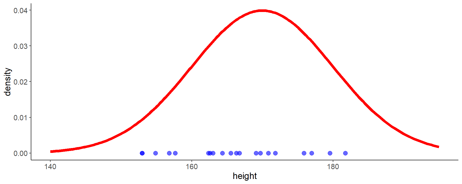
Code
ggplot(aes(x = height, y = 0), data = df) +
  geom_line(aes(y = density), data = dens_df,
            color = "red", linewidth = 2) +
  geom_segment(aes(x = height, xend = height, y = 0, yend = density),
               data = filter(likelihood_df, height == min(height)),
               color = "grey") +
  geom_segment(aes(x = height, xend = 140, y = density, yend = density),
               data = filter(likelihood_df, height == min(height)),
               color = "grey")  +
  geom_point(size = 3, color = "blue", alpha = 0.6) +
  labs(y = "density")
Code
ggplot(aes(x = height, y = 0), data = df) +
  geom_line(aes(y = density), data = dens_df,
            color = "red", linewidth = 2) +
  geom_segment(aes(x = height, xend = height, y = 0, yend = density),
               data = likelihood_df,
               color = "grey") +
  geom_segment(aes(x = height, xend = 140, y = density, yend = density),
               data = likelihood_df,
               color = "grey")  +
  geom_point(size = 3, color = "blue", alpha = 0.6) +
  labs(y = "density")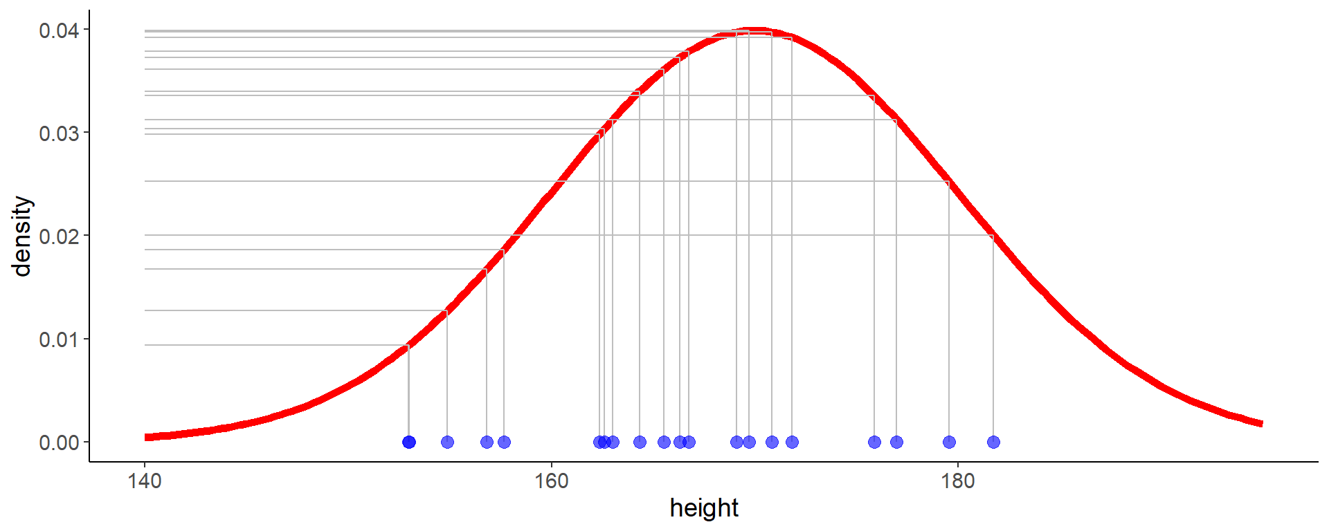
19 Likelihood for different \(\mu\) and \(\sigma\)
Code
likelihoods_df <-
  expand_grid(
    mu = seq(130, 200, length = 400),
    sigma = seq(0.1, 50, length = 400)) %>%
  mutate(log_likelihood = map2_dbl(
    mu, sigma,
    ~ sum(dnorm(heights, mean = .x, sd = .y, log = T)))) %>%
  filter(log_likelihood >= quantile(log_likelihood, 0.5))

ggplot(likelihoods_df) +
  geom_contour_filled(aes(mu, sigma, z = log_likelihood)) +
  labs(x = "mean μ", y = "standard deviation σ", fill = "log-likelihood") +
  annotate("point", x = mean(heights), y = sd(heights),
           color = "red", size = 4) +
  guides(fill = guide_legend(reverse = TRUE))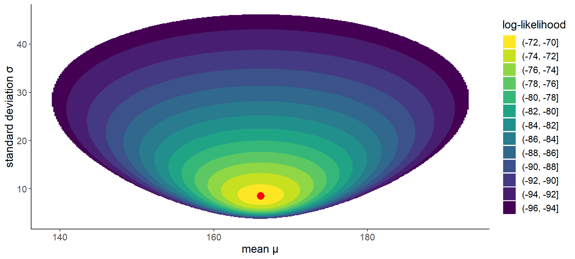
Note
The maximum likelihood estimate for a Normal distribution is the sample mean and sample standard deviation.