library(tidyr)
library(dplyr)
library(ggplot2)
library(readr)
library(forcats)
library(ggfortify)
library(MASS)

## theme for ggplot
theme_set(theme_classic())
theme_update(text = element_text(size = 14))GLMs for count and proportion data
Day 8
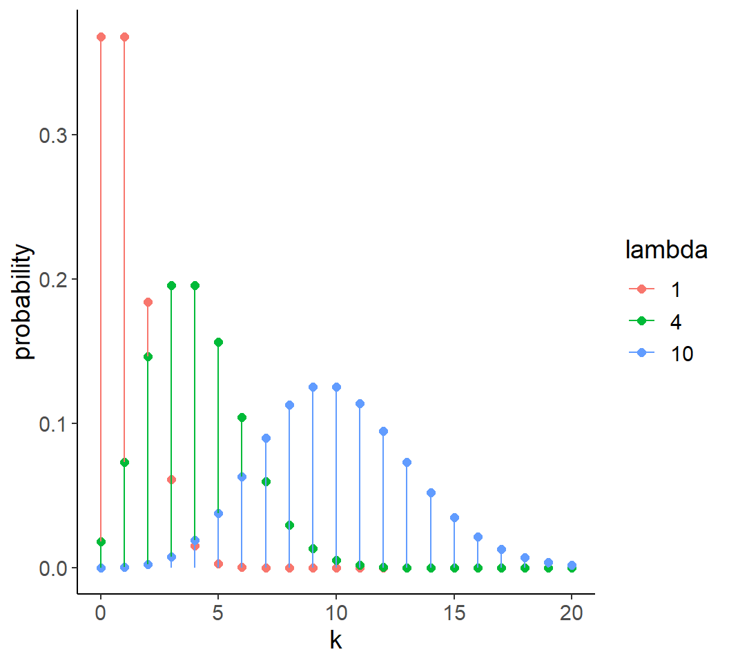
Count data
- Often described by Poisson distribution
- Discrete values and bounded:
- Y > 0
- \(\text{mean}(Y) = \text{var}(Y) = \lambda\)
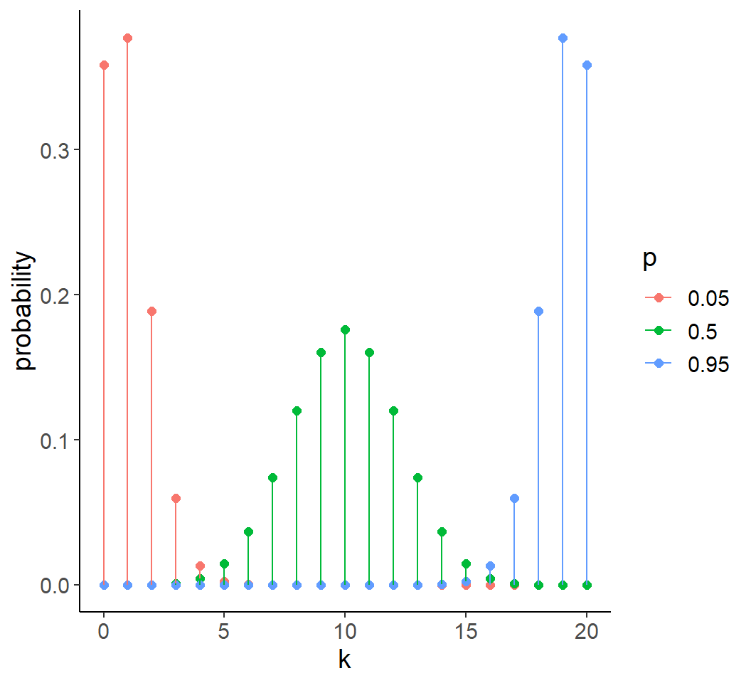
Proportion and binary data
- Often described by Binomial distribution
- Discrete values and bounded in interval [0, 1]
- \(\text{mean}(Y) = Np\)
- \(\text{var}(Y) = Np(1-p) = Np - Np^2\)
Assumptions of Linear Models
- Linear relationship between X and Y
- Normally distributed errors (residuals)
- Errors & response are not bounded \([-\infty, \infty]\)
- Constant variance of the residuals
- No relationship between mean(Y) and var(Y)
Linear models not appropriate for count, proportion and binary data!
The idea of GLMs
- Move from distributions to models
- The mean of the response \(y_i\) for data point \(i\) varies as (non-linear) function of the explanatory variables \(X_j\)
- Count data
- \(\lambda_i = f(X_j)\)
Code
soil_moisture <- runif(n = 50, min = 10, max = 50)

a <- -2
b <- 0.1
lin_pred <- a + soil_moisture*b
lambda <- exp(lin_pred)

y <- rpois(length(lambda), lambda = lambda)

dat1 <- tibble(soil_moisture,
               no_of_seedlings = y)

ggplot(dat1, aes(soil_moisture, no_of_seedlings)) +
  geom_point(size = 3, col = "seagreen") +
  xlab("Soil moisture") +
  ylab("No. of seedlings") +
  geom_smooth(method = "glm", method.args = list(family = "poisson"),
              color = "red")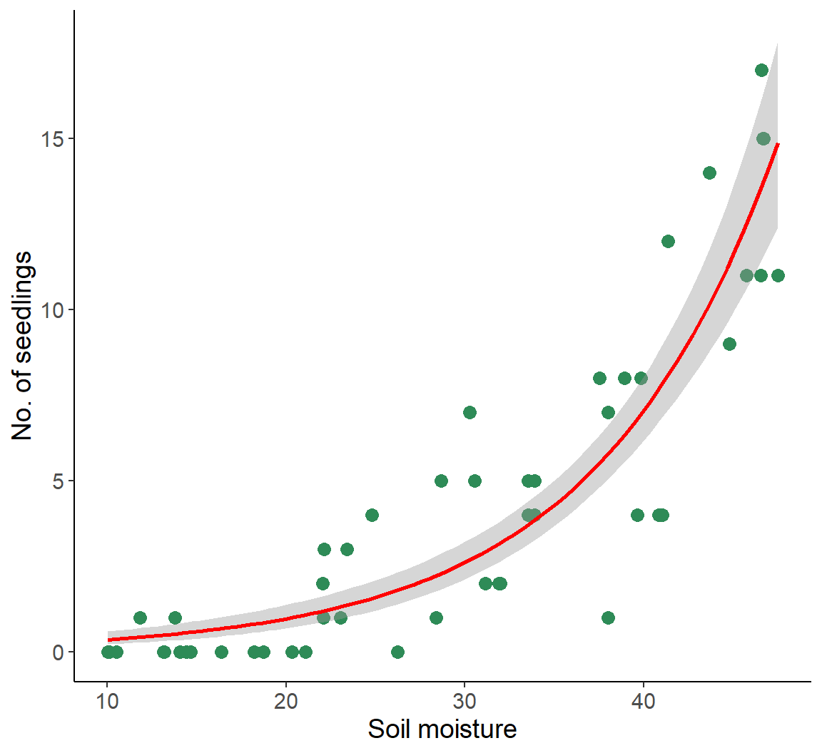
The idea of GLMs
- Proportion data
- \(p_i = f(X_j)\)
- \(N\) is defined by the data (see examples)
Code
no_of_seeds <- rep(seq(10, 100, by = 10), each = 6)

a <- 7
b <- -0.12
lin_pred <- a + no_of_seeds*b
pi <- exp(lin_pred)/(1 + exp(lin_pred))

y <- rbinom(length(pi), size = no_of_seeds, prob = pi)

dat1 <- tibble(no_of_seeds,
               no_of_seedlings = y) %>%
  mutate(prop_germinated = no_of_seedlings / no_of_seeds)

ggplot(dat1, aes(no_of_seeds, prop_germinated)) +
  geom_point(size = 3, col = "skyblue3") +
  xlab("No. of seeds") +
  ylab("Proportion of germinated seeds") +
  ggtitle("Density dependent germination rate") +
  geom_smooth(method = "glm", method.args = list(family = "binomial"),
              color = "red")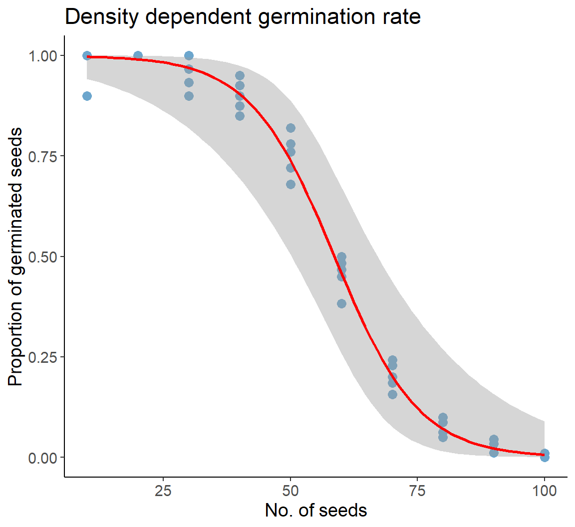
Count data: log-link function
Code
dat <- tibble(x = seq(0,10, by = 0.01),
              y = log(x))
ggplot(dat, aes(x,y)) +
  geom_line() +
  ggtitle("η = log(𝛌)") +
  theme(plot.title = element_text(hjust = 0.5)) +
  geom_hline(yintercept = 0, linetype = 2) +
  geom_vline(xintercept = 0, linetype = 2) +
  xlab("𝛌 - mean response") +
  ylab("η - linear predictor")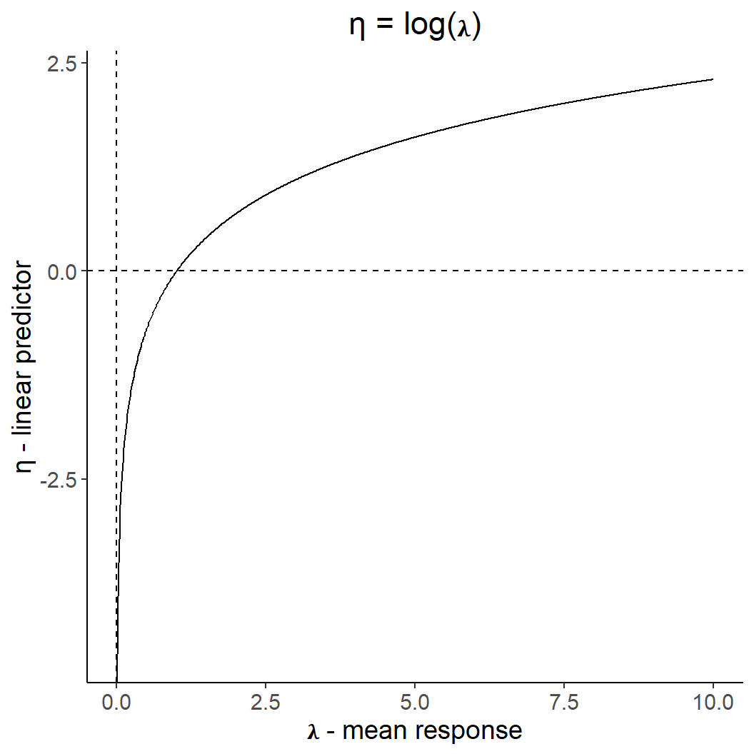
Code
dat <- tibble(x = seq(-2,4, by = 0.01),
              y = exp(x))
ggplot(dat, aes(x,y)) +
  geom_line() +
  ggtitle("𝛌 = exp(η)") +
  theme(plot.title = element_text(hjust = 0.5)) +
  geom_hline(yintercept = 0, linetype = 2) +
  geom_vline(xintercept = 0, linetype = 2) +
  xlab("η - linear predictor" ) +
  ylab("𝛌 - mean response")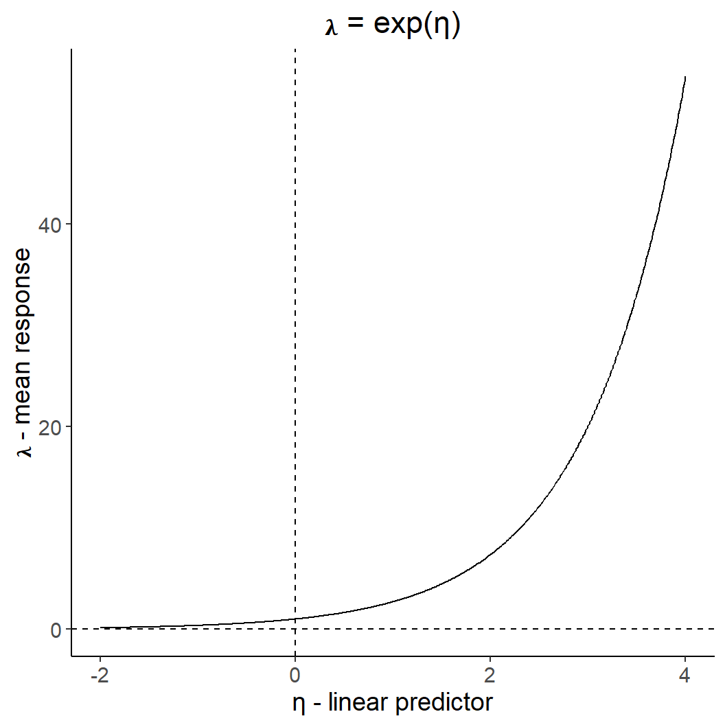
Proportion/ binary data: logit-link
Code
dat <- tibble(p = seq(0,1, by = 0.001),
              y = log(p / (1 - p)))
ggplot(dat, aes(p,y)) +
  geom_line() +
  ggtitle("η = logit(p) = log(p / (1 - p))") +
  theme(plot.title = element_text(hjust = 0.5)) +
  geom_hline(yintercept = 0, linetype = 2) +
  geom_vline(xintercept = 0, linetype = 2) +
  xlab("p - mean response") +
  ylab("η - linear predictor")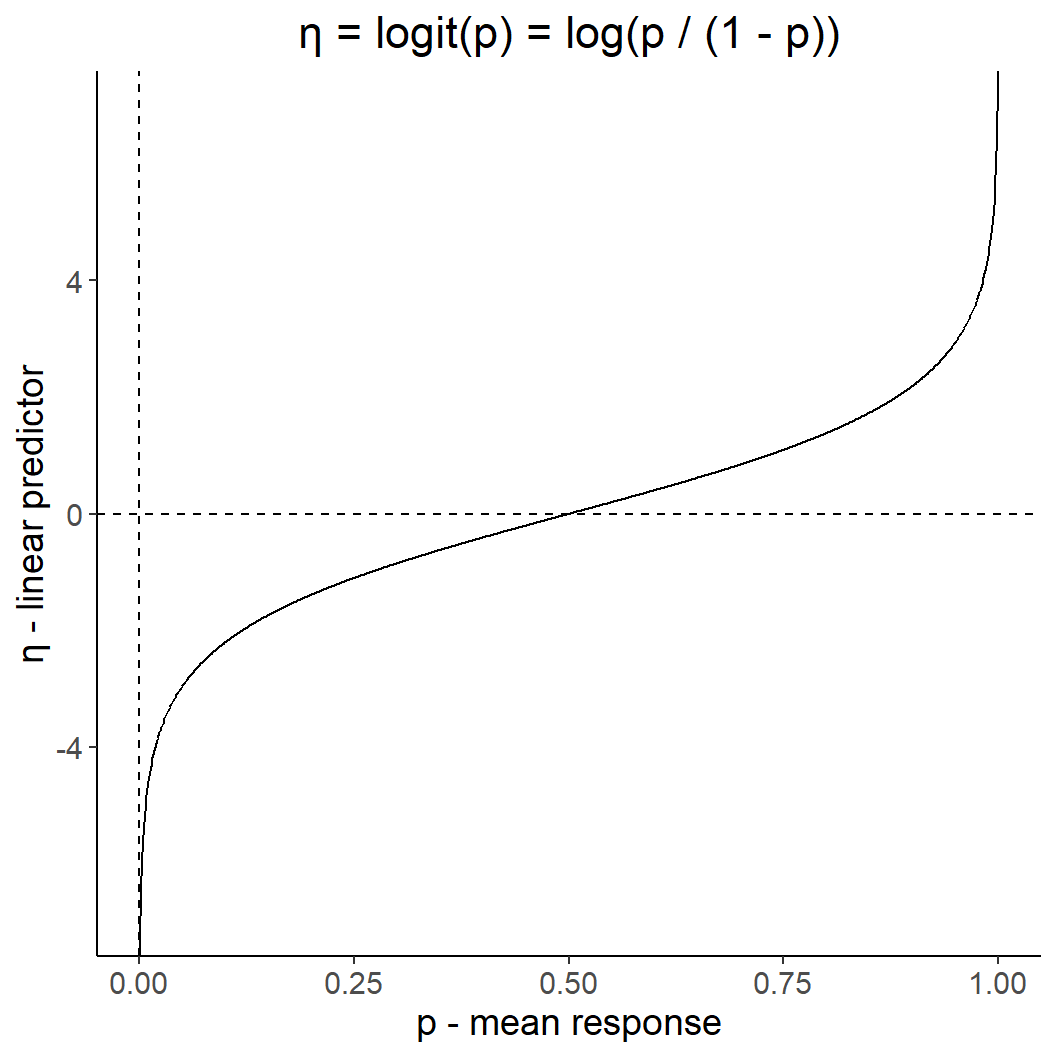
Code
dat <- tibble(y = seq(-5,5, by = 0.01),
              p = exp(y)/(1 + exp(y)))
ggplot(dat, aes(y,p)) +
  geom_line() +
  ggtitle("p = exp(η)/(1 + exp(η))") +
  theme(plot.title = element_text(hjust = 0.5)) +
  geom_hline(yintercept = 0, linetype = 2) +
  geom_vline(xintercept = 0, linetype = 2) +
  xlab("η - linear predictor" ) +
  ylab("p - mean response")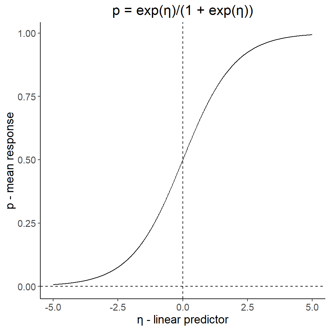
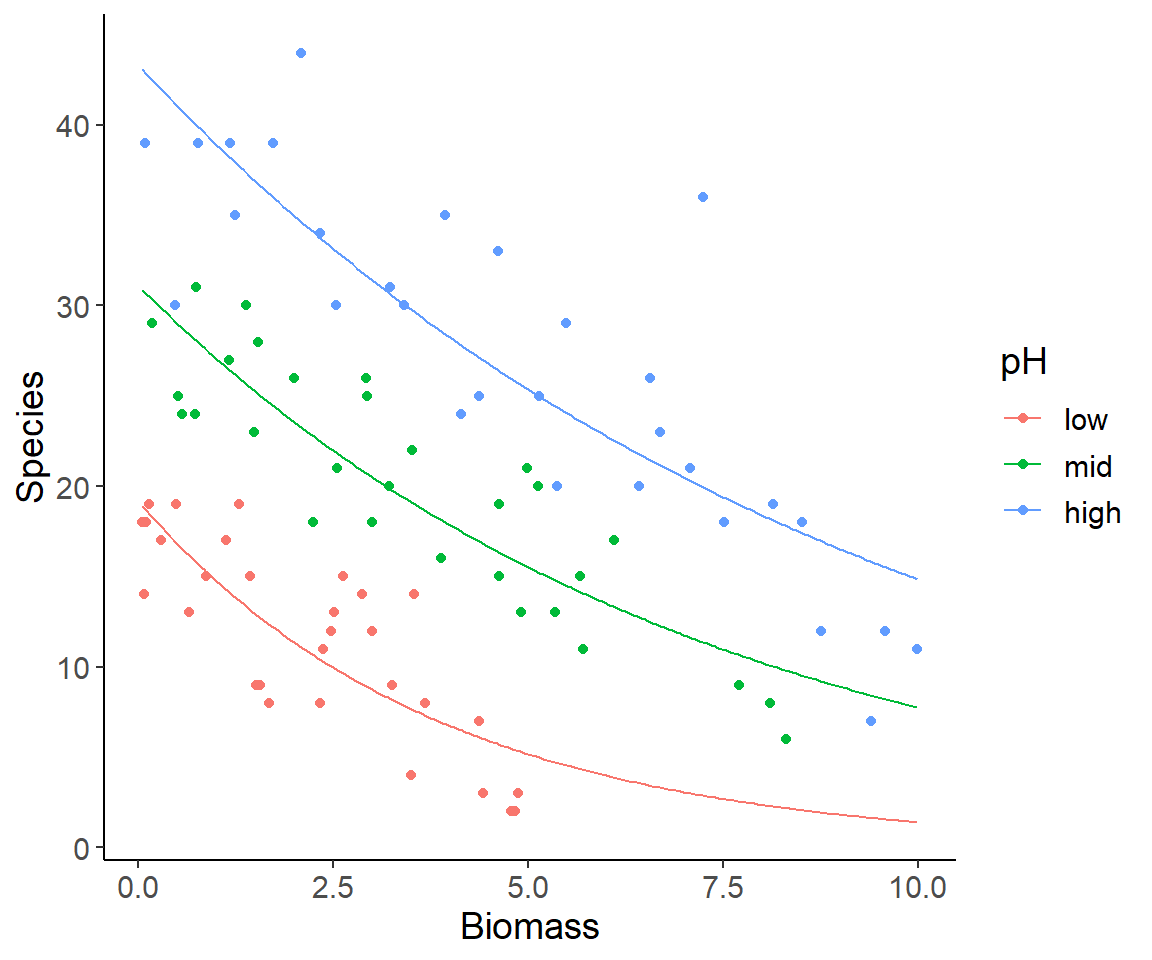
Poisson GLM in R
- Check and prepare the data
- What do you dislike about this plot?
specdat <- read_csv("data/08_species.csv")
ggplot(specdat, aes(Biomass, Species, color = pH)) +
  geom_point(size = 2.5)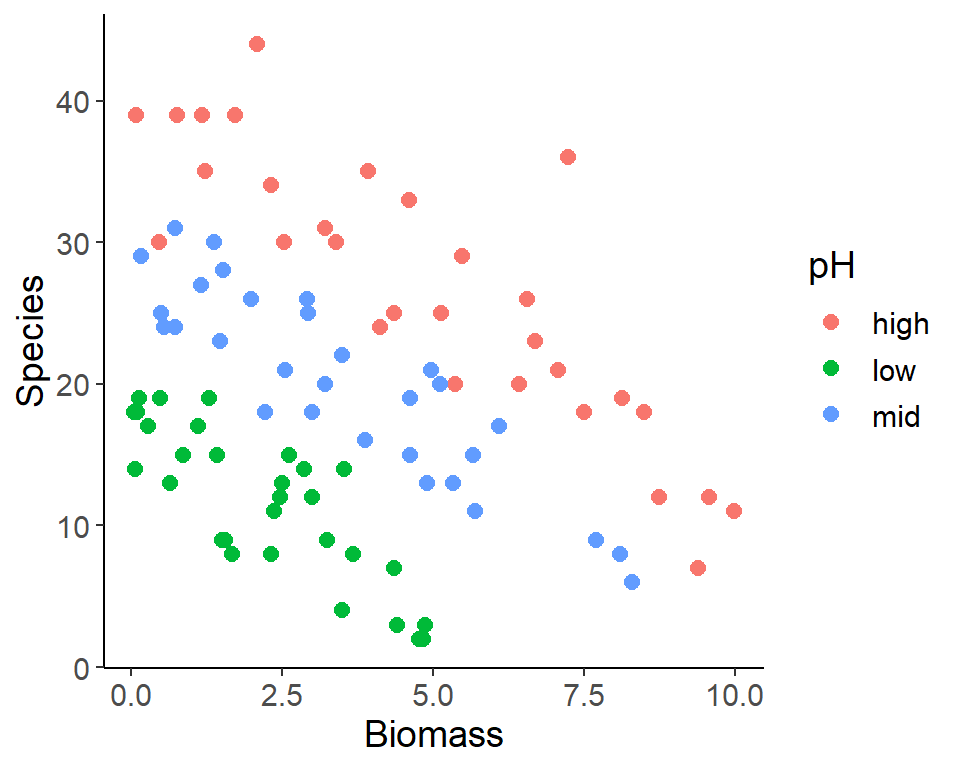
Adjusting factor levels
- Intuitive order of a categorical variable / factor
specdat <- specdat %>%
  mutate(pH = fct_relevel(pH, "low", "mid", "high"))

ggplot(specdat, aes(Biomass, Species, color = pH)) +
  geom_point(size = 2.5)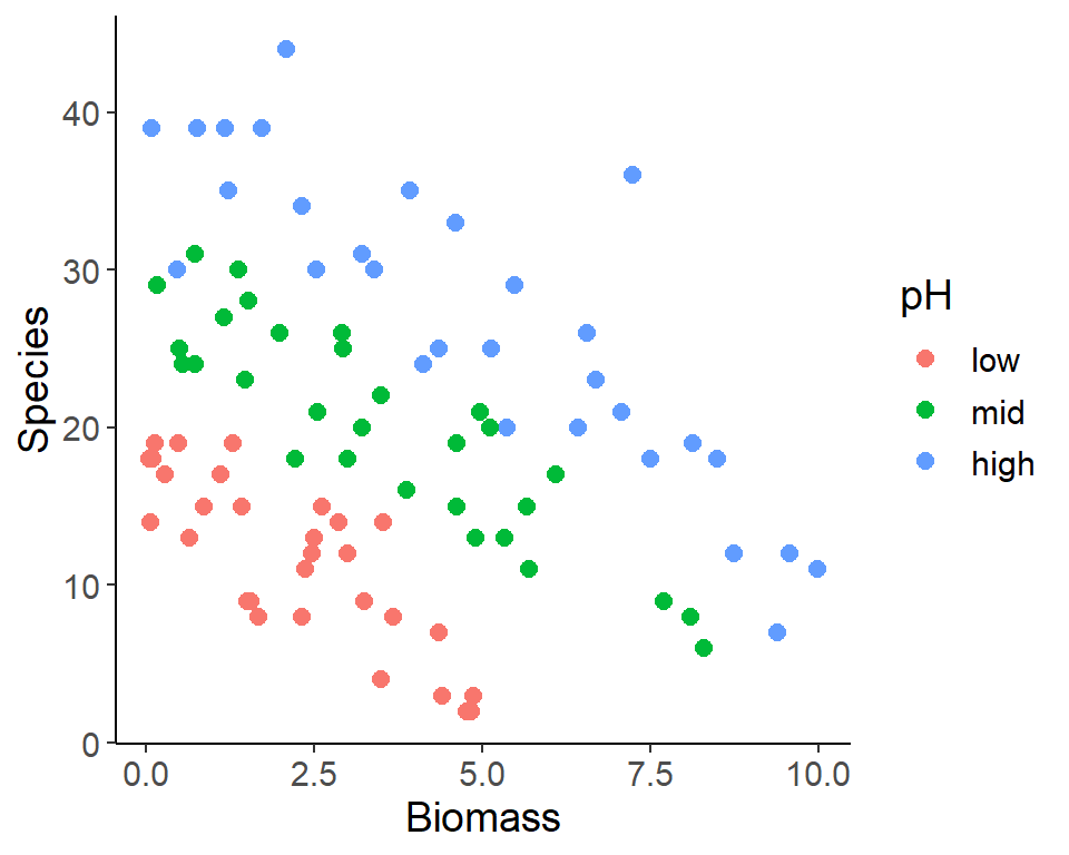
Interpret GLM summary
Call:
glm(formula = Species ~ Biomass * pH, family = "poisson", data = specdat)

Coefficients:
               Estimate Std. Error z value Pr(>|z|)
(Intercept)     2.95255    0.08240  35.833  < 2e-16 ***
Biomass        -0.26216    0.03803  -6.893 5.47e-12 ***
pHmid           0.48411    0.10723   4.515 6.34e-06 ***
pHhigh          0.81557    0.10284   7.931 2.18e-15 ***
Biomass:pHmid   0.12314    0.04270   2.884 0.003927 **
Biomass:pHhigh  0.15503    0.04003   3.873 0.000108 ***
---
Signif. codes:  0 '***' 0.001 '**' 0.01 '*' 0.05 '.' 0.1 ' ' 1

(Dispersion parameter for poisson family taken to be 1)

    Null deviance: 452.346  on 89  degrees of freedom
Residual deviance:  83.201  on 84  degrees of freedom
AIC: 514.39

Number of Fisher Scoring iterations: 4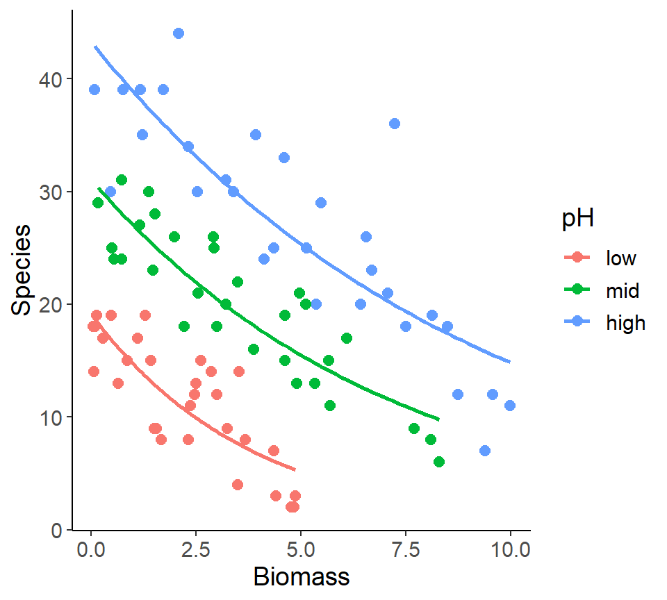
Check model assumptions
- Same interpretation as in linear models
- But: different type of residuals
autoplot(mod1)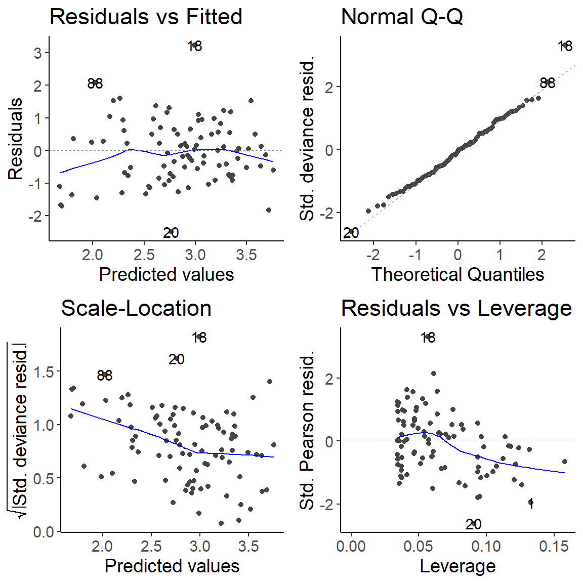
Plot the predictions
ggplot(specdat, aes(Biomass, Species, color = pH)) +
  geom_point() +
  geom_line(aes(Biomass, mean_spec), data = pred_dat)