library(tidyr)
library(dplyr)
library(ggplot2)
library(readr)
library(forcats)

## theme for ggplot
theme_set(theme_classic())
theme_update(text = element_text(size = 14))
Overdispersion in GLMs
Day 8
Overdispersion
- Poisson GLM
\(\text{mean}(y_i) = \lambda_i\)
\(\text{var}(y_i) = \lambda_i\)
\(\text{var}(y_i) > \lambda_i\)
- Binomial GLM
\(\text{mean}(y_i) = N_i p_i\)
\(\text{var}(y_i) = N_i p_i (1 - p_i)\)
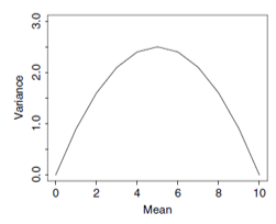
\(\text{var}(y_i) > N_i p_i (1 - p_i)\)
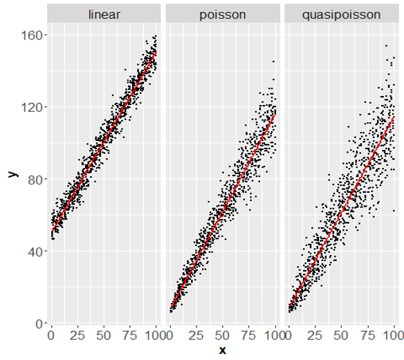
Overdispersion: Higher variance than expected from error distribution
Quasi-Likelihood approach
- Linear regression
- \(\sigma^2 = c\)
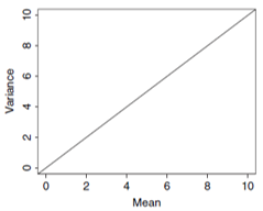
- Poisson GLM
- \(\sigma^2 = \lambda\)
- Quasipoisson GLM
- \(\sigma^2 = \phi\lambda\)
Negative binomial distribution
Code
x <- 0:25
ypois1 <- dpois(x, lambda = 10)
ynegbinom1 <- dnbinom(x, size = 4, mu = 10)
ynegbinom2 <- dnbinom(x, size = 400, mu = 10)

dat1 <- data.frame(x = rep(x, times = 2),
                   Probability = c(ypois1, ynegbinom1, ypois1, ynegbinom2),
                   Distribution = rep(rep(c("Poisson","Neg. binom"),
                                          each = length(x)), 2),
                   Theta = rep(c(4,400), each = 2*length(x)))

ggplot(dat1, aes(x, Probability, color = Distribution)) +
  geom_point(size = 2) +
  geom_line(linetype = 2) +
  facet_wrap(~Theta, labeller = label_both)
- \(\mu = 10\) in all panels
- What are the variances (according to previous slide)?
:::
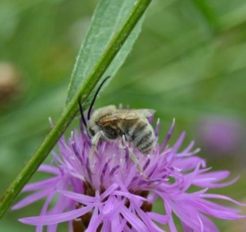
Insect diversity in urban grasslands
Inspired by FU project Flowering campus
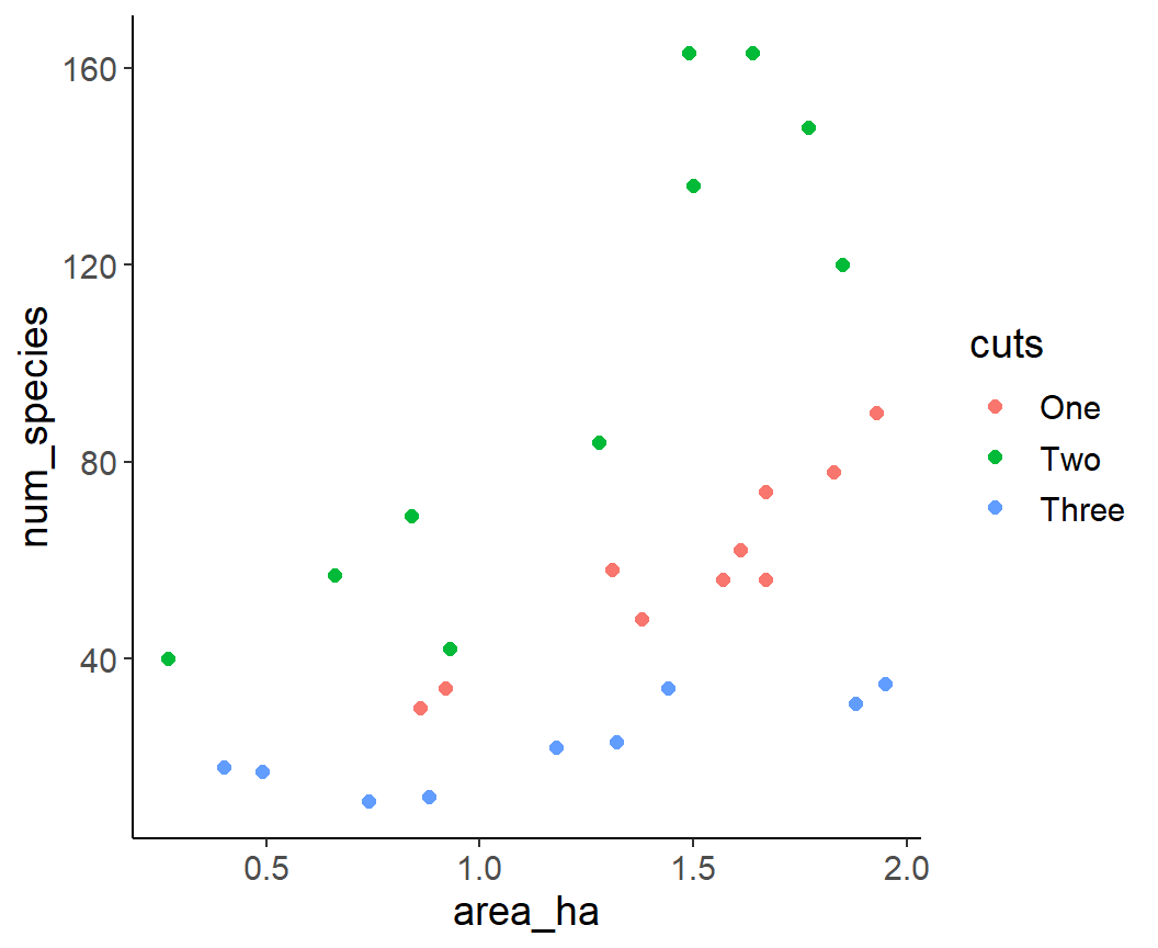
Question: How does insect species number vary with mowing frequency and area of the grassland sites?
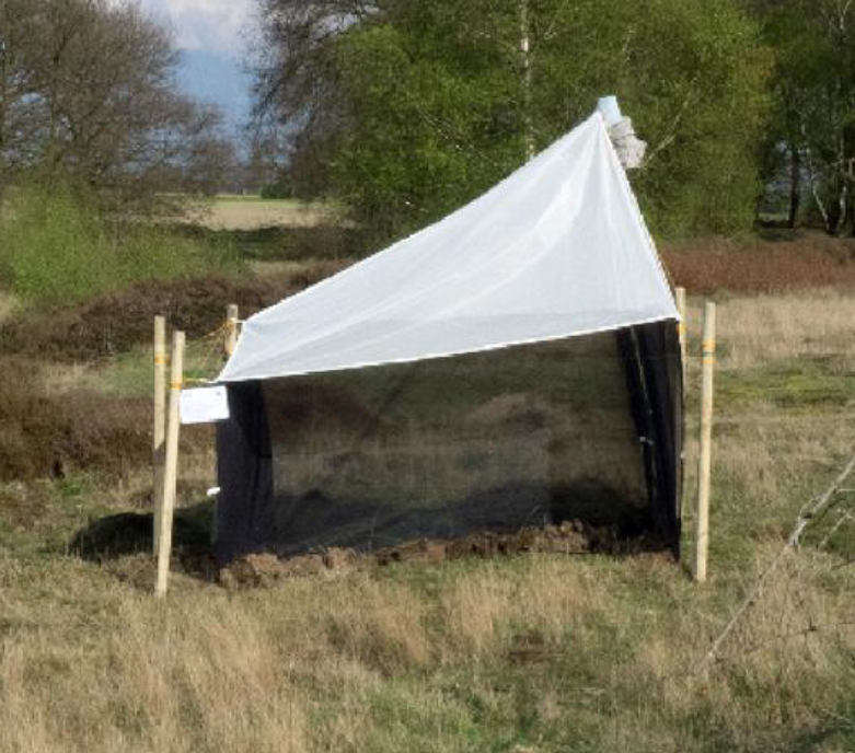
Data set: samples from 30 grassland sites
08_insect_diversity.csvVariables:
cuts:number of mowing events per year (consider as categorical variable!)area_ha:area of the grassland site in hectarnum_species:total number of insect species over the catching period
Read and plot
insects1 <- read_csv("data/08_insect_diversity.csv")
insects1
# A tibble: 30 × 3
cuts area_ha num_species
<chr> <dbl> <dbl>
1 One 1.67 74
2 One 1.38 48
3 One 1.83 78
4 One 1.57 56
5 One 1.61 62
6 One 0.86 30
7 One 1.67 56
8 One 1.31 58
9 One 1.93 90
10 One 0.92 34
# ℹ 20 more rowsggplot(insects1, aes(area_ha, num_species, color = cuts )) +
geom_point(size = 2)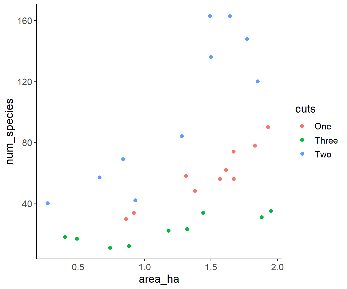
Adjust categorical variable
insects1 <- insects1 %>%
mutate(cuts = fct_relevel(cuts, "One", "Two", "Three"))
ggplot(insects1, aes(area_ha, num_species, color = cuts )) +
  geom_point(size = 2)