GLM example for proportion data

Day 8

Felix May

Freie Universität Berlin @ Theoretical Ecology

Reproduce slides

library(tidyr)
library(dplyr)
library(ggplot2)
library(readr)

## theme for ggplot
theme_set(theme_classic())
theme_update(text = element_text(size = 14))

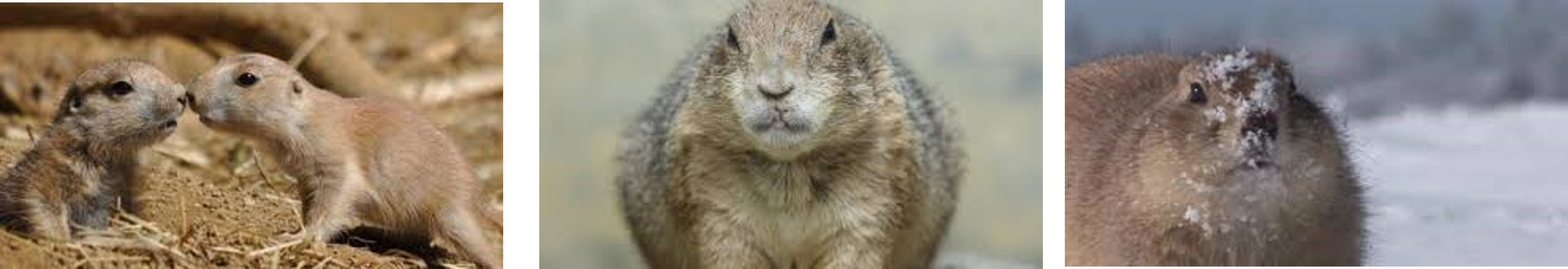
Example from animal ecology

  • Winter mortality of black tailed prairie dogs
  • Research question: How do …
    1. Successful mating
    2. Achievement of a certain minimum weight before winter
    3. Hibernation
  • … affect the probability of survival or death in winter?

Introduction of the data set

Read the data
pdogs1 <- read_csv("data/08_prairiedogs.csv")
pdogs1 %>% knitr::kable()
mated hibernation min.weight n.tot n.death
No Yes Yes 60 5
Yes Yes Yes 17 2
No No Yes 8 1
Yes No Yes 2 0
No Yes No 187 35
Yes Yes No 85 13
No No No 51 15
Yes No No 23 8

Explore the data

  • 8 rows only
  • 3 explanatory variables
    1. mated
    2. hibernation
    3. min.weight
  • What is the response here?
# A tibble: 8 × 5
  mated hibernation min.weight n.tot n.death
  <chr> <chr>       <chr>      <dbl>   <dbl>
1 No    Yes         Yes           60       5
2 Yes   Yes         Yes           17       2
3 No    No          Yes            8       1
4 Yes   No          Yes            2       0
5 No    Yes         No           187      35
6 Yes   Yes         No            85      13
7 No    No          No            51      15
8 Yes   No          No            23       8

Calculate the response

  • Proportion data –> response: proportion of surviving (or dead) animals
  • Calculate the number and proportion of survivors in R
pdogs1 <- pdogs1 %>%
  mutate(n.surv = n.tot - n.death,
         p.surv = n.surv / n.tot,
          # or alternatively
         p.dead = 1 - p.surv
  )
  • What is the problem here?

Weights of data points

  • Calculation of proportions –> loss of information
    • 2 survivors / 4 total = 50%
    • 100 survivors / 200 total = 50%
  • But: 100 out of 200 –> more information than 2 out of 4
  • Data points with higher total number –> more weight in model fitting and inference
  • Use \(N_{Total}\) as weight in GLMs

Binomial GLM for proportion data

  • Binomial GLM
    • Linear predictor: \(\eta_i = \alpha + \sum{\beta_j x_{i,j}}\)
    • Link function: \(\text{logit}(p_i) = \log\left(\frac{p_i}{1 - p_i}\right) = \eta_i\)
    • Inverse link function: \(p_i = \frac{exp(\eta_i)}{1 + exp(\eta_i)}\)
    • Binomial error distribution

Binomial GLM in R

  • Definition of the response in binomial GLMs
  • Two options:
    1. Response: proportion of successes and \(N_{Total}\) as weights
    2. Response: table with two columns
      1. No. of “successes” (here: no. of surviving animals)
      2. No. of “failures” (here: no. of dead animals)
mod1 <- glm(p.surv ~ hibernation,
            data = pdogs1,
            family = binomial,
            weights = n.tot)
mod2 <- glm(cbind(n.surv, n.death) ~ hibernation,
            data = pdogs1,
            family = binomial)

Apply graphics and GLMs

  • How do …
    1. Successful mating
    2. Achievement of a certain minimum weight before winter
    3. Hibernation
  • … affect the probability of survival or death in winter?
  • Evidence for important two-way interactions?
  • Evidence for important main effects?

Explore interactions

  • Example: Interactive effects of mating and hibernation on survival?
  • How would you plot this?
ggplot(pdogs1, aes(x = hibernation, y = p.surv,
                   fill = mated)) + 
  geom_boxplot() +
  xlab("Hibernation") + ylab("Proportion survivors")

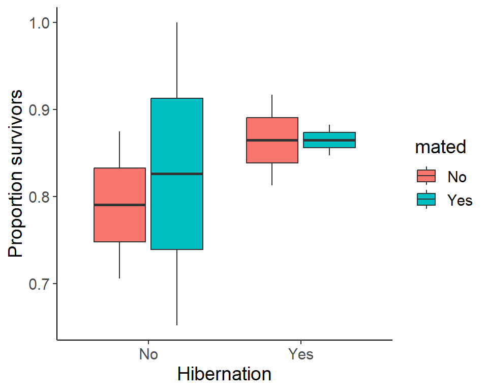
Explore main effects

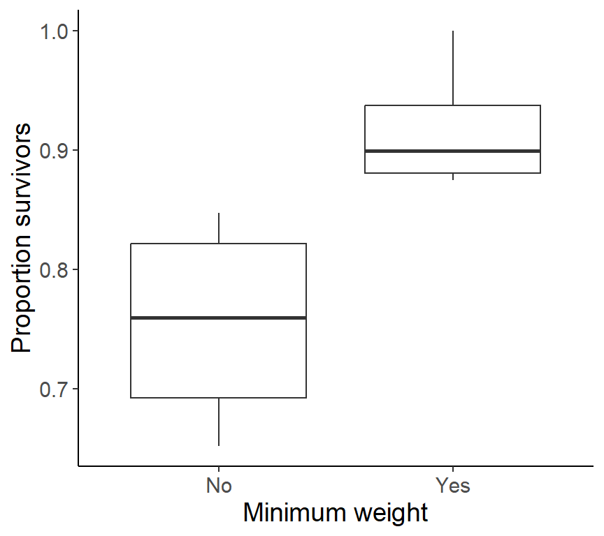
  • Example: Main effect of minimum weight?
ggplot(pdogs1, aes(x = min.weight, y = p.surv)) + 
  geom_boxplot() +
  xlab("Minimum weight") + ylab("Proportion survivors")

Exercise

  • Check all possible two-way interactions
  • Check all possible main-effects
  • With graphics
  • With models