This vignette shows how to classify landscape patterns using a convolutional neural network (Keras backend) trained directly on landscape raster data.
The workflow consists of the following steps:
- Generate training landscapes with known patterns using the
create_landscapes()function. - Train a neural network on the landscape pixel data using the
train_nn_pixels()function. - Classify new landscapes using the trained model with the
apply_nn_pixels()function.
Setup Keras
Models are trained using the R package keras3. It requires a working installation of TensorFlow.
You can refer to our installation guide and the official keras3 package website for instructions on how to install Keras and TensorFlow.
To quickly test if your setup is working, you can run the following simple function from the keras3 package:
keras3::to_categorical(0)
#>      [,1]
#> [1,]    1
If the function does not return an error, your Keras installation is working correctly.
Set seed for reproducibility
Keras models do not use R’s random number generator (RNG). Therefore, it is not enough to set a seed with set.seed(). To set both a seed for R and for Keras RNG, you can use the set_random_seed() function from spatPatClassifyR.
set_random_seed(123456)Step 1: Generate Training Landscapes
You can generate a set of training landscapes with known patterns. See landscape generation vignette for details on landscape generation and available patterns and options.
training_landscapes <- create_landscapes(
  n = 100,
  patterns = c("labyrinth", "random", "clustered")
)
#> ✔ Successfully generated all 100 training landscapes
Step 2: Train Neural Network
The model can be trained with or without cross-validation. Valid methods for the cross-validation method cv_method are:
-
"none": No cross-validation, train on all data. -
"k-fold": k-fold cross-validation withcv_foldsnumber of folds. -
"loo": leave-one-out cross-validation.
For details and further options see the function help of train_nn_pixels().
The underlying model uses a multiscale convolutional neural network (CNN) architecture that processes the landscapes as 2D pixel arrays. The model layers multiple convolutional layers with different kernel sizes (3 x 3 and 5 x 5) to capture both fine-scale details and broader spatial patterns. The architecture consists of paired convolutional layers, followed by pooling to reduce dimensionality and a final dense layer for the classification. The user can specify various parameters for training the model, such as the learning rate, the number of epochs and patience, but also for validating the model, such as the cross-validation method (k-fold or leave-one-out) and the proportion of validation data.
Here, we train the model using 2-fold cross-validation to keep computational time low.
Low fold accuracy
The function will print fold accuracies during training (see below). If the accuracy is low, consider increasing the number of training landscapes or check the function help for other options to improve model performance.
model <- train_nn_pixels(
  landscapes = training_landscapes,
  cv_method = "k-fold",
  cv_folds = 2,
  verbose = FALSE
)
To check the model performance, we can look at the confusion matrix from cross-validation:
# Confusion matrix from cross-validation
model$performance$confusion_matrix
#>            Actual
#> Predicted   clustered labyrinth random
#>   clustered        27         6      0
#>   labyrinth         6        27      0
#>   random            0         1     33
You can also check other performance metrics like overall accuracy:
# Overall accuracy
model$performance$accuracy
#> [1] 0.87
Or per class metrics like precision, recall, and F1-score:
model$performance$per_class_metrics
#> # A tibble: 3 × 5
#>   class     count recall precision f1_score
#>   <chr>     <int>  <dbl>     <dbl>    <dbl>
#> 1 clustered    33   0.82      0.82     0.82
#> 2 labyrinth    34   0.79      0.82     0.81
#> 3 random       33   1         0.97     0.99
Step 3: Classify New Landscapes
Finally, you can create some new test landscapes and classify them using the trained model. In this example, we create 20 new landscapes for testing.
In reality this could be landscapes read in from files or created in other ways. For details on importing own landscapes, see the importing landscapes vignette.
test_landscapes <- create_landscapes(
  n = 20,
  patterns = c("labyrinth", "random", "clustered")
)
#> ✔ Successfully generated all 20 training landscapes
If test landscapes have been created with create_landscapes(), their true patterns are known. Therefore they can be used to evaluate classification performance.
Note
To get additional performance metrics, set
return_performance = TRUEwhen applying the model. This only works if true patterns are known. If true patterns are not known, setreturn_performance = FALSE(default).
classification <- apply_nn_pixels(
  landscapes = test_landscapes,
  nn_model = model,
  return_performance = TRUE
)
You can look at the predicted patterns for each test landscape individually and compare actual and predicted classes:
# Predicted patterns
classification$predictions
#> # A tibble: 20 × 8
#>    landscape_id landscape_name actual_class predicted_class confidence clustered
#>           <int> <chr>          <chr>        <chr>                <dbl>     <dbl>
#>  1            1 random_1       random       random               1.000 1.17 e- 9
#>  2            2 labyrinth_2    labyrinth    labyrinth            1.000 1.89 e- 5
#>  3            3 random_3       random       random               1     6.91 e-13
#>  4            4 random_4       random       random               1     8.03 e-19
#>  5            5 random_5       random       random               1     5.63 e-18
#>  6            6 random_6       random       random               1     1.86 e-16
#>  7            7 random_7       random       random               1.000 9.30 e-11
#>  8            8 clustered_8_r… clustered    clustered            0.993 9.93 e- 1
#>  9            9 labyrinth_9    labyrinth    labyrinth            1.000 5.76 e- 6
#> 10           10 clustered_10_… clustered    clustered            0.974 9.74 e- 1
#> 11           11 clustered_11_… clustered    clustered            1.000 1.000e+ 0
#> 12           12 labyrinth_12   labyrinth    labyrinth            0.999 7.10 e- 4
#> 13           13 labyrinth_13   labyrinth    labyrinth            1.000 5.52 e- 5
#> 14           14 labyrinth_14   labyrinth    labyrinth            1.000 6.92 e- 7
#> 15           15 labyrinth_15   labyrinth    clustered            0.926 9.26 e- 1
#> 16           16 labyrinth_16   labyrinth    labyrinth            1.000 5.84 e- 7
#> 17           17 clustered_17_… clustered    clustered            1.000 1.000e+ 0
#> 18           18 clustered_18_… clustered    clustered            1.000 1.000e+ 0
#> 19           19 clustered_19_… clustered    clustered            1.000 1.000e+ 0
#> 20           20 random_20      random       random               1     1.50 e-15
#> # ℹ 2 more variables: labyrinth <dbl>, random <dbl>
You can also look at performance summaries like confusion matrix:
# Performance summary
classification$performance$confusion_matrix
#>            Actual
#> Predicted   clustered labyrinth random
#>   clustered         6         1      0
#>   labyrinth         0         6      0
#>   random            0         0      7
And other metrics like accuracy, precision, recall, and F1-score:
# Other performance metrics
classification$performance$per_class_metrics
#> # A tibble: 3 × 5
#> class count recall precision f1_score
#> <chr> <int> <dbl> <dbl> <dbl>
#> 1 clustered 6 1 0.86 0.92
#> 2 labyrinth 7 0.86 1 0.92
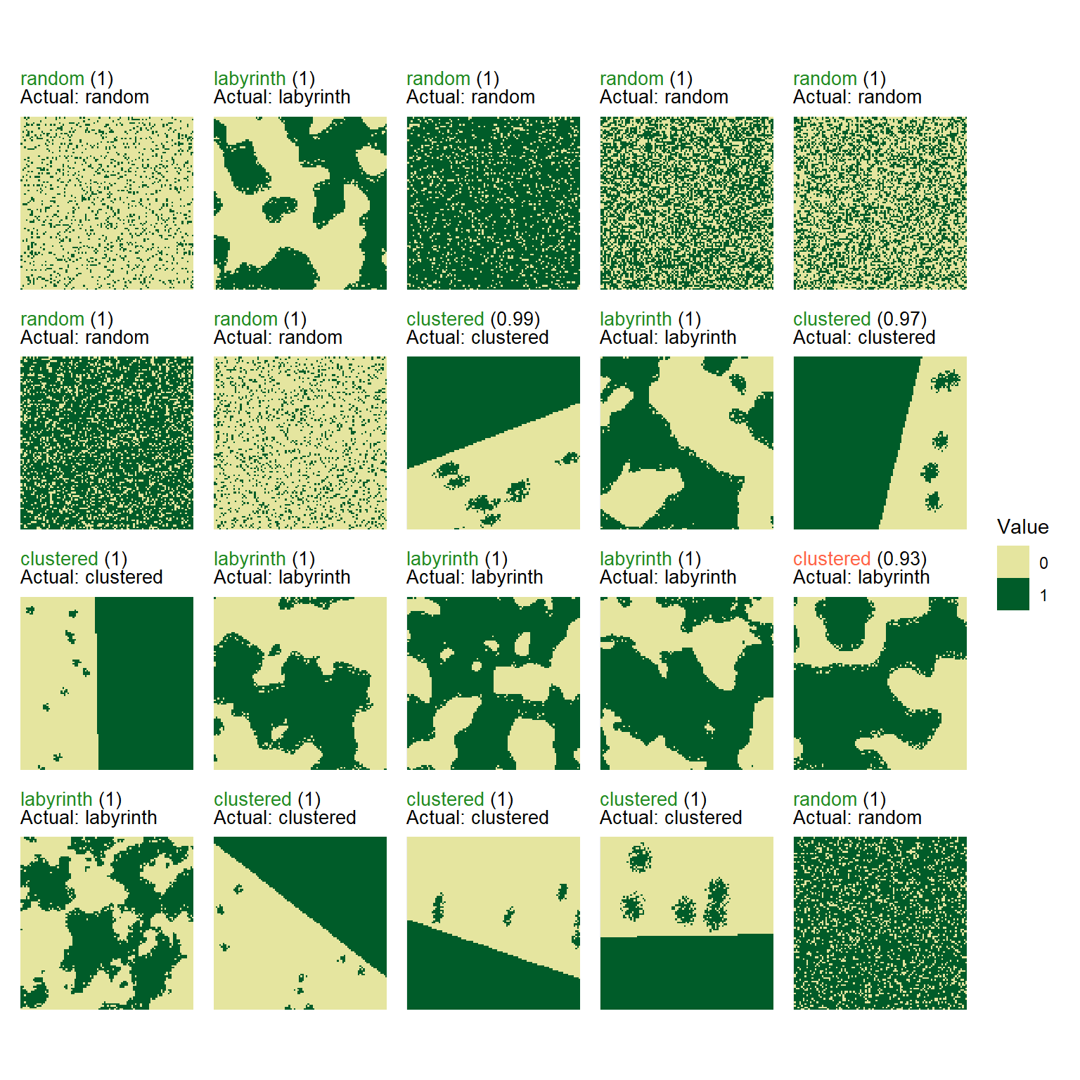
#> 3 random 7 1 1 1To visualize the classified landscapes along with their true and predicted patterns use the function plot_classified_landscapes. Correctly classified landscapes are shown in green, misclassified ones in red. To plot only misclassified landscapes, set only_misclassified = TRUE.
Note
If you classified landscapes where the true patterns are not known, the plot will show the landscape and the predicted pattern only.
# Visualize true and predicted patterns

plot_classified_landscapes(
  classification = classification$predictions,
  landscapes = test_landscapes
)