Pattern gallery • patternscaper

This gallery provides an overview of the 11 spatial patterns available for artificial landscapes, organized into control, ecotone, and patch patterns. The examples show how selected parameters affect their appearance. To see all parameters for a specific pattern, open the corresponding help page, for example ?pattern_spots.

See Create artificial landscapes for instructions on generating individual landscapes and training batches.

library(patternscaper)
# Set seed for reproducible examples
set.seed(123456)

Control patterns

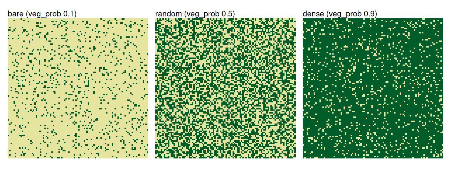
The patterns bare, random, and dense place vegetation at random. They differ only in veg_prob, the probability that each cell is vegetated: bare defaults to 0.1, random to 0.5, and dense to 0.9. These patterns provide control landscapes without a specific spatial structure.

bare <- create_landscape("bare", name = "bare (veg_prob 0.1)")
random <- create_landscape("random", name = "random (veg_prob 0.5)")
dense <- create_landscape("dense", name = "dense (veg_prob 0.9)")

list(bare, random, dense) |>
  plot_landscapes(
    titles = "name",
    show_legend = FALSE
  )

Three landscapes showing control patterns: bare, random, and dense

Ecotone patterns

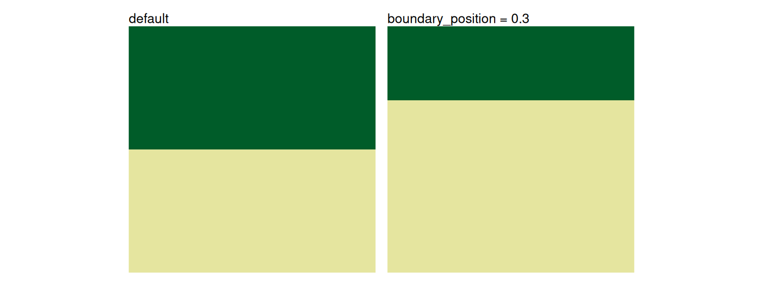
Ecotone patterns have a vegetated zone and a bare zone with a transition between them. In an unrotated landscape, the parameter boundary_position gives the relative position of this transition measured from the top. It applies to all five ecotone patterns.

Sharp

An abrupt boundary, with boundary_position as its only parameter.

list(
  create_landscape("sharp", name = "default"),
  create_landscape(
    "sharp",
    name = "boundary_position = 0.3",
    params = pattern_sharp(boundary_position = 0.3)
  )
) |>
  plot_landscapes(
    titles = "name",
    show_legend = FALSE
  )

Two sharp-boundary landscapes: default and boundary position 0.3

Diffuse

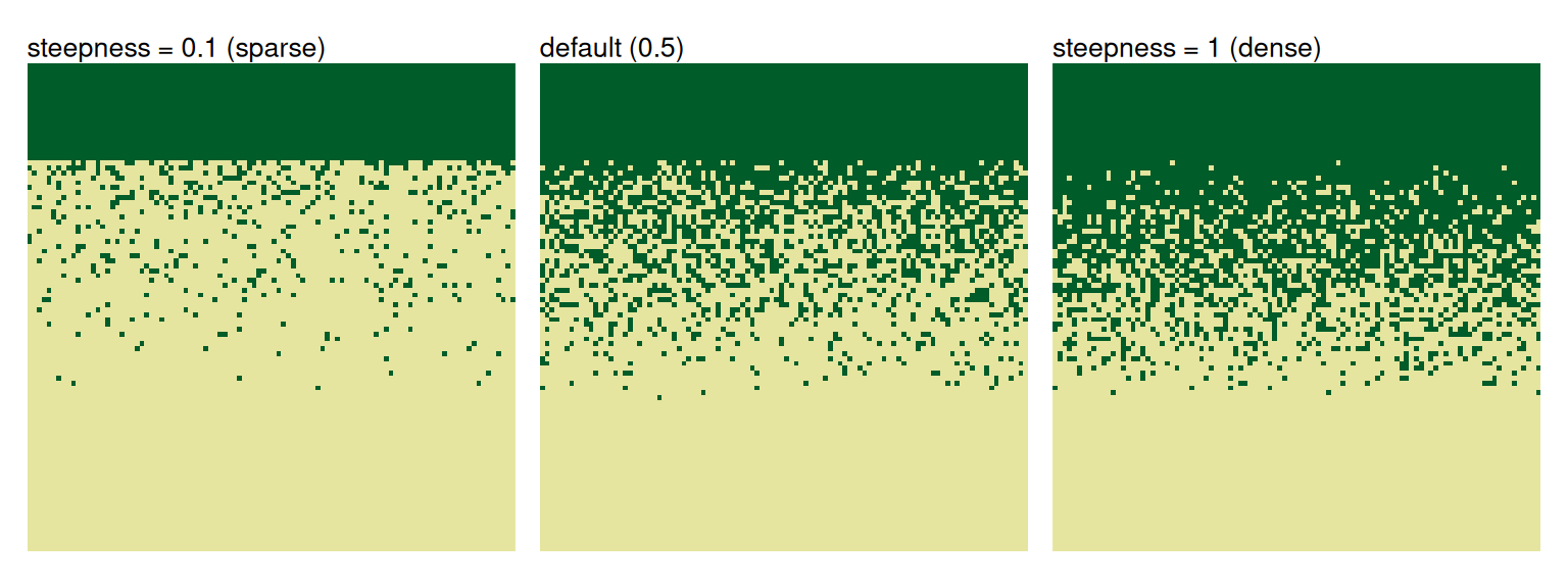
A transition where vegetation probability decreases with distance below the boundary. steepness controls how quickly that probability drops: values near 0 produce a sparse, abrupt transition, while values near 1 produce a denser, more gradual transition. The potential extent of the transition remains unchanged.

list(
  create_landscape(
    "diffuse",
    name = "steepness = 0.1 (sparse)",
    params = pattern_diffuse(steepness = 0.1)
  ),
  create_landscape("diffuse", name = "default (0.5)"),
  create_landscape(
    "diffuse",
    name = "steepness = 1 (dense)",
    params = pattern_diffuse(steepness = 1)
  )
) |>
  plot_landscapes(
    titles = "name",
    show_legend = FALSE
  )

Three diffuse-boundary landscapes with increasingly dense transition zones

Fingers

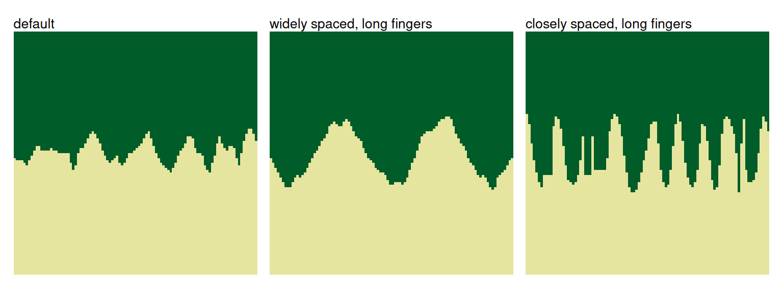
Curved, finger-like extensions of vegetation into the bare zone. The parameter sine_length_mean controls the average wavelength of the curves (larger values result in more widely spaced fingers). The parameter sine_height_mean controls the average finger amplitude (larger values result in longer fingers). The corresponding *_sd parameters control the variation between fingers.

list(
  create_landscape("fingers", name = "default"),
  create_landscape(
    "fingers",
    name = "widely spaced, long fingers",
    params = pattern_fingers(
      sine_length_mean = 40,
      sine_height_mean = 12
    )
  ),
  create_landscape(
    "fingers",
    name = "closely spaced, long fingers",
    params = pattern_fingers(
      sine_length_mean = 10,
      sine_height_mean = 15,
      sine_height_sd = 3
    )
  )
) |>
  plot_landscapes(
    titles = "name",
    show_legend = FALSE
  )

Three finger landscapes: default, widely spaced long fingers, and closely spaced long fingers

Clustered

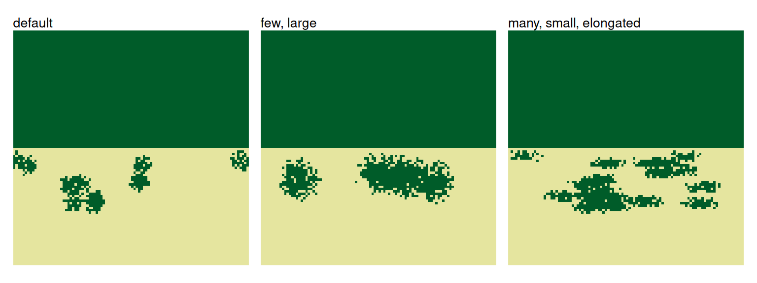
Vegetation clusters scattered below the vegetation boundary in the bare zone. n_clusters and cluster_radius set cluster number and size, cluster_zone controls how far into the bare zone they can occur, and elongation_x and elongation_y stretch them along either axis.

list(
  create_landscape("clustered", name = "default"),
  create_landscape(
    "clustered",
    name = "few, large",
    params = pattern_clustered(n_clusters = 5, cluster_radius = 10)
  ),
  create_landscape(
    "clustered",
    name = "many, small, elongated",
    params = pattern_clustered(
      n_clusters = 20,
      cluster_radius = 3,
      elongation_x = 3
    )
  )
) |>
  plot_landscapes(
    titles = "name",
    show_legend = FALSE
  )

Three clustered landscapes: default, few large clusters, and many small elongated clusters

Bands

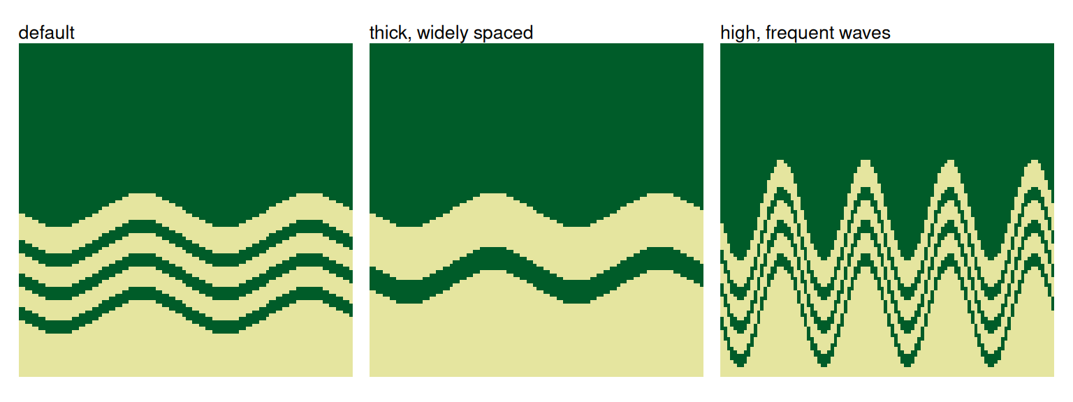
Sinusoidal vegetation bands parallel to the vegetation boundary. band_thickness sets band thickness, band_spacing the distance between bands, amplitude their wave height, and frequency how often their waves repeat across the landscape.

list(
  create_landscape("bands", name = "default"),
  create_landscape(
    "bands",
    name = "thick, widely spaced",
    params = pattern_bands(band_thickness = 6, band_spacing = 20)
  ),
  create_landscape(
    "bands",
    name = "high, frequent waves",
    params = pattern_bands(amplitude = 15, frequency = 0.25)
  )
) |>
  plot_landscapes(
    titles = "name",
    show_legend = FALSE
  )

Three banded landscapes: default, thick widely spaced bands, and bands with high, frequent waves

Patch patterns

Patch patterns are self-organized patterns without a boundary between two zones.

Spots

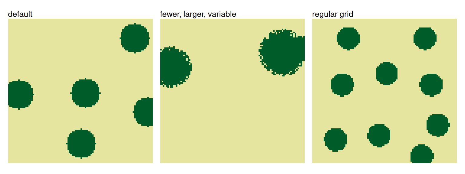
Circular vegetation patches on bare ground. n_spots and spot_radius set the count and size, spot_radius_sd varies the size between spots, radius_noise_fraction makes the spot edges rough, and regular_spots = TRUE places them on a grid instead of at random.

list(
  create_landscape("spots", name = "default"),
  create_landscape(
    "spots",
    name = "fewer, larger, variable",
    params = pattern_spots(
      n_spots = 3,
      spot_radius = 12,
      spot_radius_sd = 3,
      radius_noise_fraction = 0.2
    )
  ),
  create_landscape(
    "spots",
    name = "regular grid",
    params = pattern_spots(
      n_spots = 9,
      spot_radius = 8,
      regular_spots = TRUE
    )
  )
) |>
  plot_landscapes(
    titles = "name",
    show_legend = FALSE
  )

Three spot landscapes: default, fewer larger variable spots, and a regular grid

Gaps

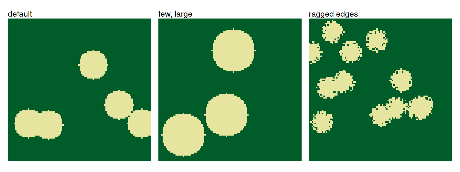
The inverse of spots: circular bare gaps in otherwise vegetated ground. It takes parameters analogous to those for spots, with names such as n_gaps and gap_radius.

list(
  create_landscape("gaps", name = "default"),
  create_landscape(
    "gaps",
    name = "few, large",
    params = pattern_gaps(n_gaps = 3, gap_radius = 15)
  ),
  create_landscape(
    "gaps",
    name = "ragged edges",
    params = pattern_gaps(
      n_gaps = 12,
      gap_radius = 8,
      radius_noise_fraction = 0.4
    )
  )
) |>
  plot_landscapes(
    titles = "name",
    show_legend = FALSE
  )

Three gap landscapes: default, few large gaps, and many gaps with ragged edges

Labyrinth

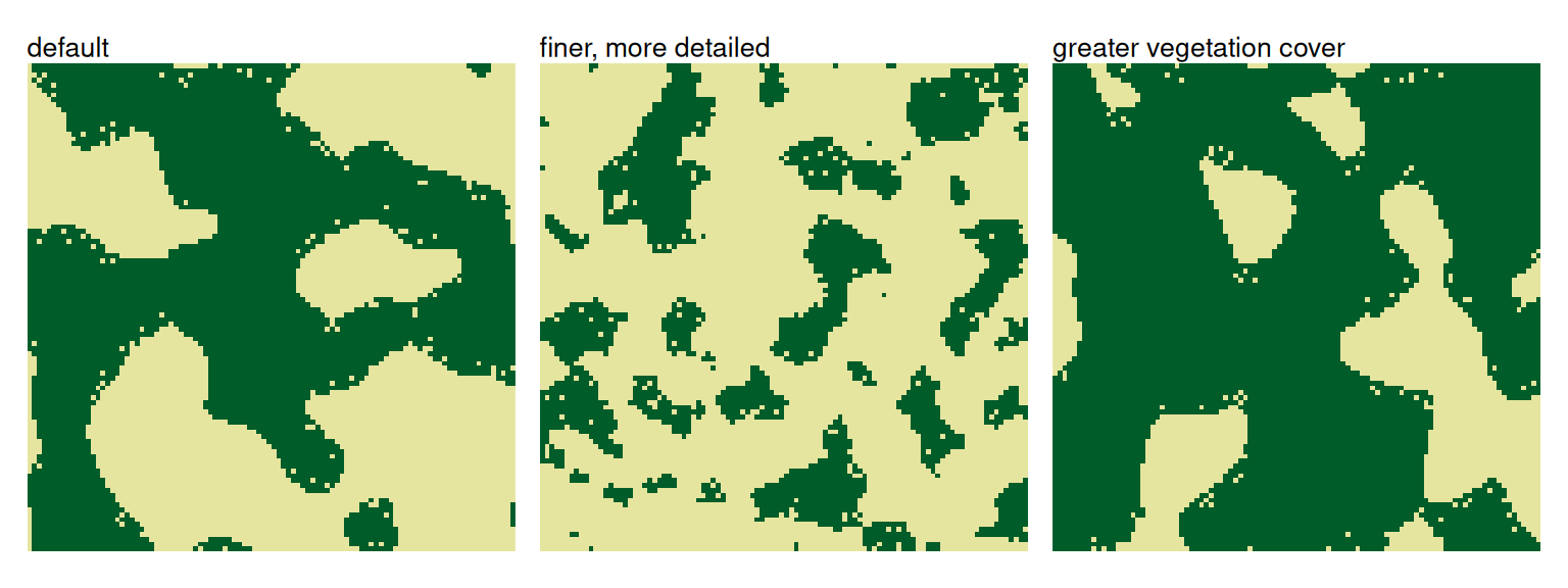
Maze-like bands of vegetation. The parameter frequency controls their dominant spatial scale, with higher values producing finer structures. The parameter octaves controls how much fine-scale detail is added, and lower veg_threshold values increase vegetation cover.

list(
  create_landscape("labyrinth", name = "default"),
  create_landscape(
    "labyrinth",
    name = "finer, more detailed",
    params = pattern_labyrinth(frequency = 6, octaves = 3)
  ),
  create_landscape(
    "labyrinth",
    name = "greater vegetation cover",
    params = pattern_labyrinth(veg_threshold = 0.35)
  )
) |>
  plot_landscapes(
    titles = "name",
    show_legend = FALSE
  )

Three labyrinth landscapes: default, a finer maze, and a labyrinth with greater vegetation cover

Next steps

Create artificial landscapes: Select patterns and generate individual landscapes or training batches