Solution for mean indicator values

1 Solution with R output

First, we read and explore the data.

library(tidyr)
library(dplyr)
library(readr)
library(ggplot2)

indi <- read_csv("data/03_ellenberg_indicator_values.csv")
veg <- read_csv("data/03_vegetation_berlin.csv")

indi

# A tibble: 123 × 7
   genus      species        light  temp moisture reaction nitrogen
   <chr>      <chr>          <dbl> <dbl>    <dbl>    <dbl>    <dbl>
 1 Acer       platanoides        4     6       NA       NA       NA
 2 Acer       pseudoplatanus     4    NA        6       NA        7
 3 Achillea   millefolium        8    NA        4       NA        5
 4 Aegopodium podagraria         5     5        6        7        8
 5 Aesculus   hippocastanum      5     6       NA       NA       NA
 6 Alliaria   petiolata          5     6        5        7        9
 7 Allium     canadense         NA    NA       NA       NA       NA
 8 Allium     schoenoprasum      7    NA       NA        7        2
 9 Allium     strictum           9     6        2        6        1
10 Alnus      glutinosa          5     5        9        6       NA
# ℹ 113 more rows

veg

# A tibble: 222 × 4
   plotID    plot_type species              cover_londo
   <chr>     <chr>     <chr>                      <dbl>
 1 Biesdorf1 half_open Achillea millefolium           4
 2 Biesdorf1 half_open Bellis perennis                2
 3 Biesdorf1 half_open Bryophyta                      4
 4 Biesdorf1 half_open Cardamine parviflora          10
 5 Biesdorf1 half_open Carex syvatica Huds.          30
 6 Biesdorf1 half_open Cynodon dactylon               4
 7 Biesdorf1 half_open Dactylis glomerata             4
 8 Biesdorf1 half_open Eranthis hyemalis             20
 9 Biesdorf1 half_open Ficaria verna                  2
10 Biesdorf1 half_open Galium album                   4
# ℹ 212 more rows

In the vegetation data there is only one column with the species name, while in the indicator dataset there is one column for the genus and one for the species. This has to match to have proper keys in the tables. The primary key is the the species in the indicator value dataset, while the foreign key is the species column in the vegetation survey dataset.

Here, we unite the genus and species columns in the indicator table, but we could also separate the species column in the vegetation table. Both approaches should work,

indi2 <- indi %>% unite("species", genus:species,  sep = " ")

Now, we check, if we have proper primary key with unique values only.

indi2 %>%
  count(species) %>%
  filter(n > 2)

# A tibble: 0 × 2
# ℹ 2 variables: species <chr>, n <int>

Now, we can join the two tables and calculate the mean indicator values for every plot. When we want to compare the plot types later, this variable also has to be included in the grouping call.

# Join the two tables by adding the indicator values to the vegetation surveys
veg2 <- veg %>%
  left_join(indi2)

# Calculate the mean indicator values for each plot
indi_mean <- veg2 %>%
  group_by(plotID, plot_type) %>%
  summarise(light_mean = mean(light, na.rm = T),
            light_mean_weighted = weighted.mean(light, cover_londo, na.rm = T))

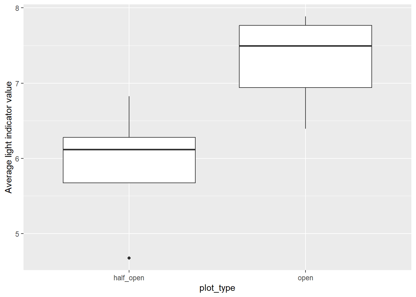
And finally, we create boxplots to compare the indicator values between the open and half-open sites

ggplot(indi_mean, aes(plot_type, light_mean_weighted)) +
  geom_boxplot() +
  ylab("Average light indicator value")

Indeed, the average light indicator value if higher in the open sites. This reflects that species on open sites are adapted to higher light availability.

2 Solution as one script without output

# Read the data
indi <- read_csv("data/03_ellenberg_indicator_values.csv")
veg <- read_csv("data/03_vegetation_berlin.csv")

# Create a single column with the species and genus names in the indicator table
# (Alternatively, you could split the single column in the vegetation dataset into two columns)
indi2 <- indi %>% unite("species", genus:species,  sep = " ")

# Check if you have a proper primary key with unique values only
indi2 %>%
  count(species) %>%
  filter(n > 2)

# Join the two tables by adding the indicator values to the vegetation surveys
veg2 <- veg %>%
  left_join(indi2)

# Calculate the mean indicator values for each plot
indi_mean <- veg2 %>%
  group_by(plotID, plot_type) %>%
  summarise(light_mean = mean(light, na.rm = T),
            light_mean_weighted = weighted.mean(light, cover_londo, na.rm = T))

# Plot the differences as boxplot
ggplot(indi_mean, aes(plot_type, light_mean_weighted)) +
  geom_boxplot() +
  ylab("Average light indicator value")