# Look at the first lines of the iris dataset
head(iris)
# What is the iris dataset -> Call the help
?iris
# How many rows and columns does the data set have?
rownum <- nrow(iris)
colnum <- ncol(iris)
print(paste0("The iris dataset has ", rownum, " rows and ", colnum, " columns."))
# Some summary statistics on the iris data set
summary(iris)

# create a plot
plot(iris$Petal.Length, iris$Petal.Width,
  xlab = "Petal Length",
  ylab = "Petal Width",
  main = "Petal Width vs Petal Length",
  pch = 20,
  col = ifelse(iris$Species == "setosa", "coral1",
    ifelse(iris$Species == "virginica", "cyan4",
      ifelse(iris$Species == "versicolor",
        "darkgoldenrod2", "grey"
      )
    )
  )
)
# add a legend
legend("bottomright", c("setosa", "virginica", "versicolor"),
  col = c("coral1", "cyan4", "darkgoldenrod2"), pch = 20
)Course Introduction
1 Lecture
1.1 General Course Introduction
1.2 R and RStudio
1.3 Read in datas and Tidyverse
2 Exercises
2.1 Change settings in RStudio
Before you get started, there is an important setting that you should change in RStudio. By default, RStudio will save the workspace of your current session in an .Rdata file. This would allow you to start the next session exactly where you left it by loading the .Rdata file.
This is not a good default. We always want to start R from a clean slate to ensure reproducibility and minimize error potential.
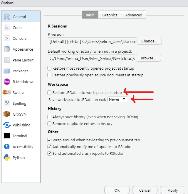
In RStudio go to Tools -> Global Options -> General and
- Remove the check mark for “Restore .RData into workspace at startup”
- Never “Save workspace to .RData on exit”
2.2 Create an RStudio project
Create an RStudio project for all the scripts, notes, data, etc. from this workshop:
- Create a project in a directory of your choice following the instructions from the slides
- Use the Files pane in RStudio to create a basic folder structure in your project which will be filled with files in the next days:
- Folder
data/for all data files - Folder
R/for all R scripts - Folder
docs/for other documents (e.g. lecture notes or slides) - You can always change the structure of your project later
You can add files to your project either directly in RStudio, or in the file explorer of your operating system.
2.2.1 Add an R script to the project
- Create a new R script and save it in the
R/folder of your project - Copy and paste the code from below into your script
- Don’t worry if you don’t understand the code yet, we will learn all this later
- Run the code in the script line by line. Try both, running code using the Run button (in the top right corner of your script pane) and the keyboard shortcut
Ctrl/Cmd + Enter- For each line that you run, observe what is happening to the different panes (console, environment, …) in RStudio. Can you explain what is happening?
2.3 Variables and vectors
Assign the value 10 to a variable x and create a vector y with the values {5, 9, 3, 4, 1000}. Now multiply these together and save the result in a new object z. Then form the sum of all elements of z.
2.4 Simple mathematical calculations
Calculate:
- \(a = 5^5\)
- \(b = \sqrt5\)
- \(c = \sqrt{5^5}\)
- \(d = \sum^4_{k=1} x_k\) with:
- \(x_1 = 5\)
- \(x_2 = 6\)
- \(x_3 = 7\)
- \(x_4 = 8\)
2.5 Vectors in R
You have the following three vectors:
species: name of the speciesbodywt_kg: body weight of the species in kgbrainwt_g: brain weight of the species in g
species <- c(
  "MountainBeaver", "Cow", "GreyWolf", "Goat",
  "GuineaPig", "Diplodocus", "AsianElephant", "Donkey",
  "Horse", "PotarMonkey", "Cat", "Giraffe",
  "Gorilla", "Human", "AfricanElephant", "Triceratops",
  "RhesusMonkey", "Kangaroo", "GoldenHamster", "Mouse",
  "Rabbit", "Sheep", "Jaguar", "Chimpanzee",
  "Rat", "Brachiosaurus", "Mole", "Pig"
)

bodywt_kg <- c(
  1.4, 465, 36.3, 27.7, 1., 11700, 2547, 187.1,
  521, 10, 3.3, 529, 207, 62, 6654, 9400,
  6.8, 35, 0.1, 0.02, 2.5, 55.5, 100, 52.2,
  0.3, 87000, 0.1, 192
)

brainwt_kg <- c(
  0.0081, 0.423, 0.1195, 0.115, 0.0055, 0.05,
  4.603, 0.419, 0.655, 0.115, 0.0256, 0.68,
  0.406, 1.32, 5.712, 0.07, 0.179, 0.056,
  0.001, 0.0004, 0.0121, 0.175, 0.157, 0.44,
  0.0019, 0.1545, 0.003, 0.18
)
Copy and paste the vectors into your R script and solve the following tasks.
- Check which of the following animals are contained in the
speciesvector:
animals_to_check <- c("Snail", "Goat", "Chimpanzee", "Rat", "Dragon", "Eagle")- Calculate mean and standard deviation of the brain weight
- Hint: have a look at the summary slides to find the functions
- Which species have a brain weight larger than the mean brain weight of all species?
- Calculate the ratio of brain weight to body weight in percent for all animals and save the result in a new vector
- A bit more tricky: Are there any animals with a larger brain to body weight ratio than humans? If yes, which ones?
- Hint: calculate the ratio for humans and save it in a separate variable first
2.6 Vectors in R: Extras
- Round the ratio vector to 4 decimal places with the
roundfunction- Type
?roundinto the console to open the help of theroundfunction
- Type
- Which animal has the smallest brain to body weight ratio?
- Hint: have a look at the
minfunction
- Hint: have a look at the
- Add the following three animals to the data vectors
species_new <- c("Eagle", "Snail", "Lion")
brainwt_kg_new <- c(0.0004, NA, 0.5)
bodywt_kg_new <- c(18, 0.01, 550)
Now calculate the mean brain weight again. Can you explain what happens? Can you fix it?
- Hint: have a look at
?mean
2.7 Read in datas
Lesen Sie den Datensatz “01_Eisbaeren.txt” ein.
2.8 Get started with readr and the tidyverse
Before you start, make sure to install the tidyverse packages by calling
install.packages("readr")This will install readr along with other tidyverse packages.
Remember to put library(tidyverse) (or library(readr)) on top of your script to access the readr functions.
2.8.1 Write a tibble to disk
Let’s use the animals tibble from the previous task and write it into the data folder in our project.
Before writing the tibble
- Create a
datasub-folder in your RStudio project (if you don’t have one yet)- Hint: You can do that from within RStudio by using the
New Folderbutton in the Files pane
- Hint: You can do that from within RStudio by using the
Now write the animals tibble into that /data sub-directory as animals.csv using a comma separator.
Check if the file was written into the correct folder.
2.9 Read data into R
Now, try to read the data set back into R using the appropriate read_* function.
Make sure that you save the table you read in in a new variable to have it available for later use.
Tip
Don’t type the input path of the table to read. Instead, make the “” to start writing the path and then us the tab key on your keyboard to auto-complete.
2.9.1 Extra
Navigate to your
data/folder using the Files pane of RStudio. Click on the.csvfile that you just saved there. What can you do? Try the Import Dataset button and see what you can do there.Try reading some
xlsxorcsvtables that you have on your machine into R- First copy the table into the
data/folder in your project, then use the appropiate function to read in the data
- First copy the table into the