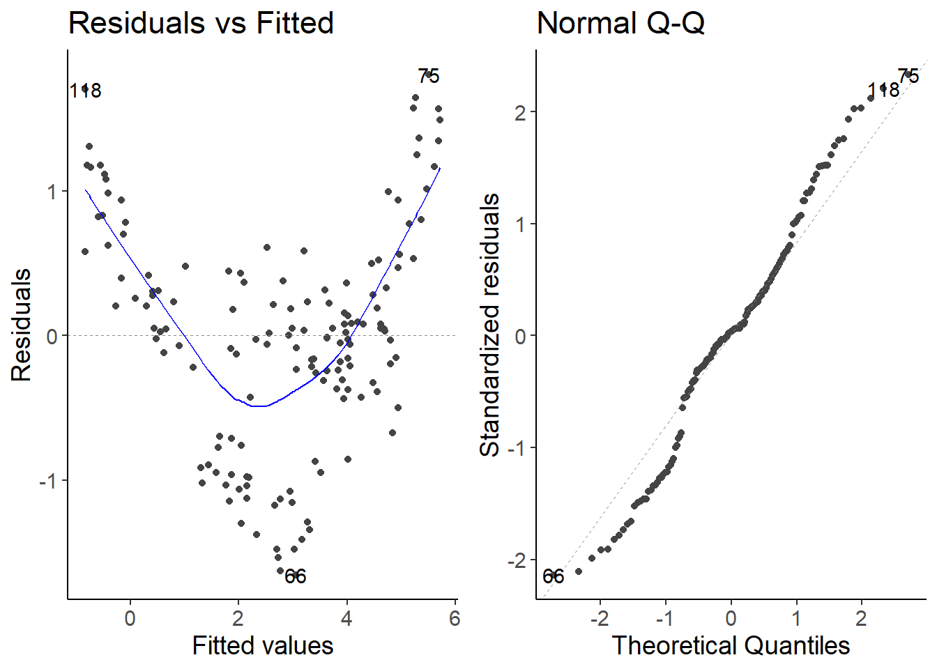
## fit model without interactionlm1 <-lm(density ~ species + temperature, data = df_bacteria)autoplot(lm1, which =1:2)
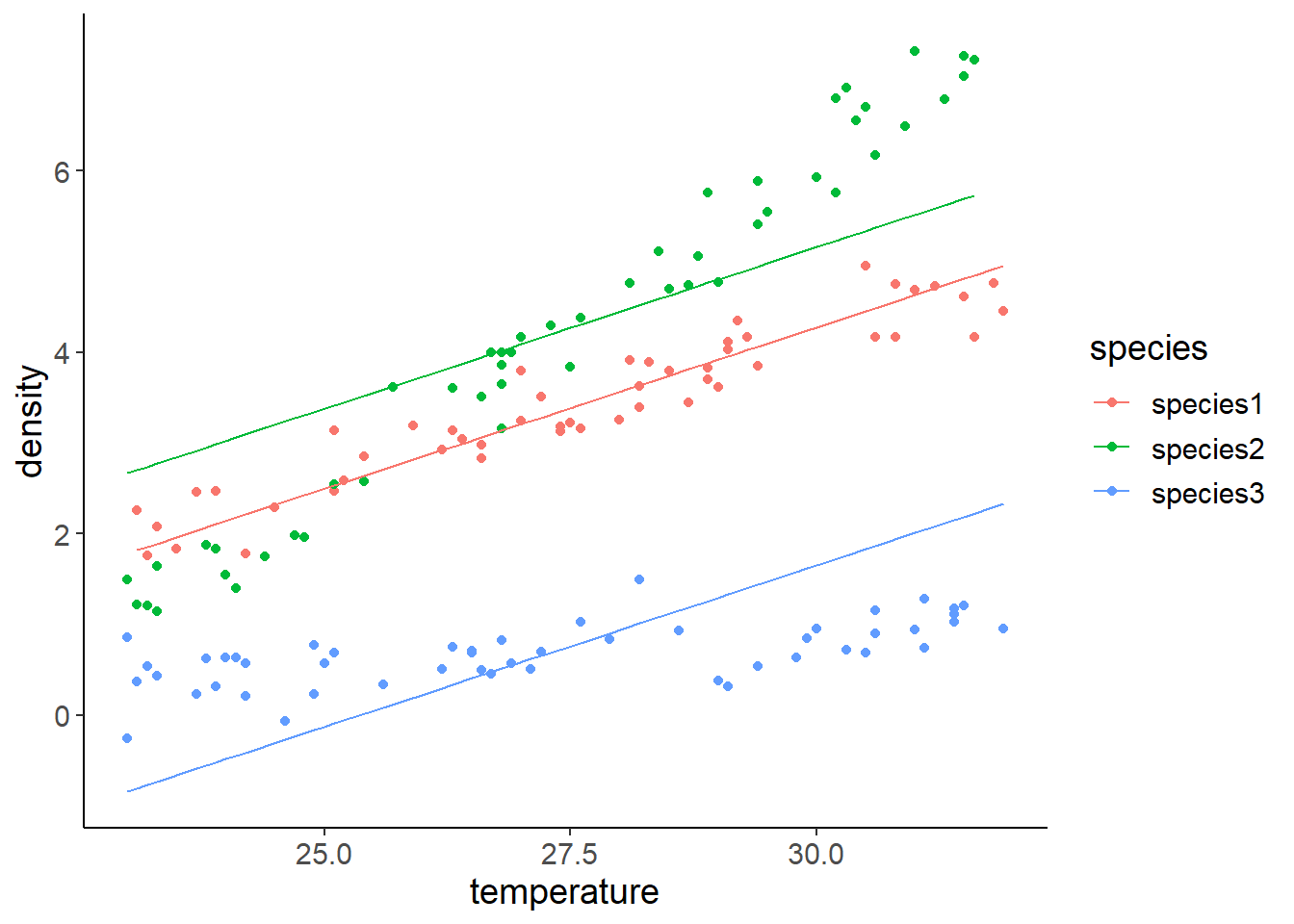
df_pred1 <-mutate(df_bacteria, density_pred =predict(lm1)) ggplot(df_pred1, aes(x = temperature, y = density, color = species)) +geom_point() +geom_line(aes(y = density_pred))
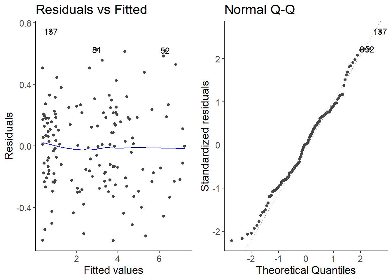
## fit model with interactionlm2 <-lm(density ~ species * temperature, data = df_bacteria)autoplot(lm2, which =1:2)
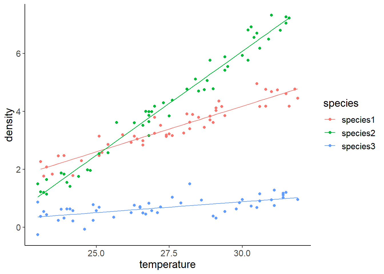
df_pred2 <-mutate(df_bacteria, density_pred =predict(lm2)) ggplot(df_pred2, aes(x = temperature, y = density, color = species)) +geom_point() +geom_line(aes(y = density_pred))
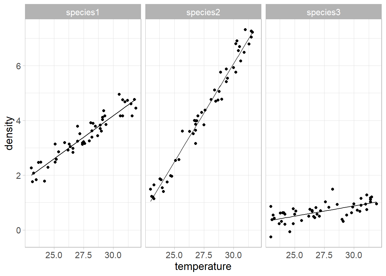
## or with facetsggplot(df_pred2, aes(x = temperature, y = density)) +geom_point() +geom_line(aes(y = density_pred)) +facet_wrap(~ species) +theme_light() +theme(text =element_text(size =14))
2 Explanation and equations
Model without interaction
lm1
Call:
lm(formula = density ~ species + temperature, data = df_bacteria)

Coefficients:
    (Intercept)  speciesspecies2  speciesspecies3      temperature
        -6.4072           0.8829          -2.6237           0.3560
The model with interaction fits much better to the data. For the model without interaction, the residuals are not normally distributed.
3 Script for copy-paste
library(dplyr)library(readr)library(ggplot2)library(ggfortify)## theme for ggplottheme_set(theme_classic())theme_update(text =element_text(size =14))df_bacteria <-read_csv("data/06_bacteria.csv")df_bacteria## fit model without interactionlm1 <-lm(density ~ species + temperature, data = df_bacteria)autoplot(lm1, which =1:2)df_pred1 <-mutate(df_bacteria, density_pred =predict(lm1)) ggplot(df_pred1, aes(x = temperature, y = density, color = species)) +geom_point() +geom_line(aes(y = density_pred)) ## fit model with interactionlm2 <-lm(density ~ species * temperature, data = df_bacteria)autoplot(lm2, which =1:2)df_pred2 <-mutate(df_bacteria, density_pred =predict(lm2)) ggplot(df_pred2, aes(x = temperature, y = density, color = species)) +geom_point() +geom_line(aes(y = density_pred)) ## or with facetsggplot(df_pred2, aes(x = temperature, y = density)) +geom_point() +geom_line(aes(y = density_pred)) +facet_wrap(~ species) +theme_light() +theme(text =element_text(size =14))