library(readr)
library(dplyr)
library(ggplot2)
library(ggfortify)
library(tidyr)

theme_set(theme_classic())
theme_update(text = element_text(size = 14))Solution to the Covid-19 in Berlin exercise
1 Load packages
2 Read data and subset to Berlin
df <- read_csv("data/07_bl_infektionen.csv") %>%
    mutate(cases7 = bl_inz) %>%
    filter(bundesland == "Berlin") %>%
    rename(date = datum) %>%
    select(date, cases7)
3 Plot the number of cases over time
ggplot(df, aes(x = date, y = cases7)) +
    geom_line(size = 1) +
    labs(x = "Date",
            y = "Reported cases of the last seven days",
title = "Reported covid cases in Berlin") 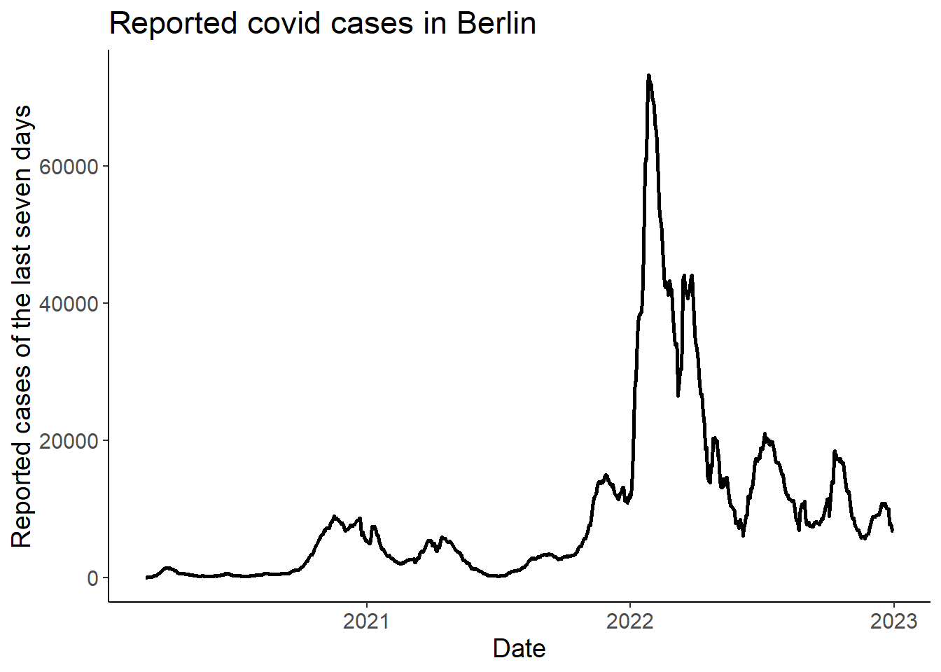
4 Fit model to first time period
first_df <- filter(df, date >= "2020-03-11" & date <= "2020-03-22" )

lm1 <- lm(cases7 ~ date, data = first_df)
autoplot(lm1, which = 1:2)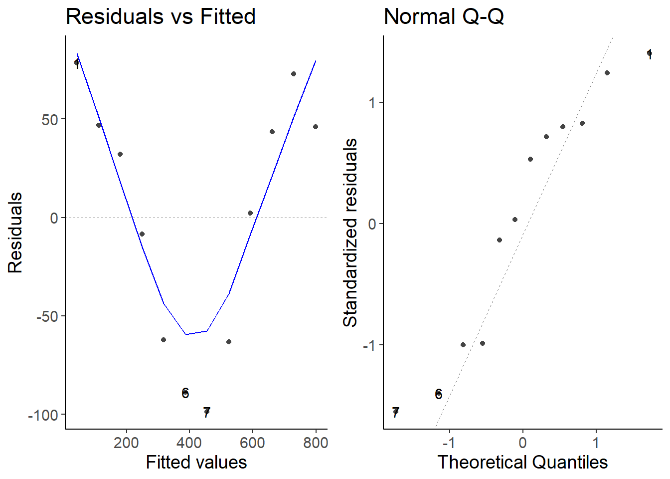
lm2 <- lm(log(cases7) ~ date, data = first_df)
autoplot(lm2, which = 1:2)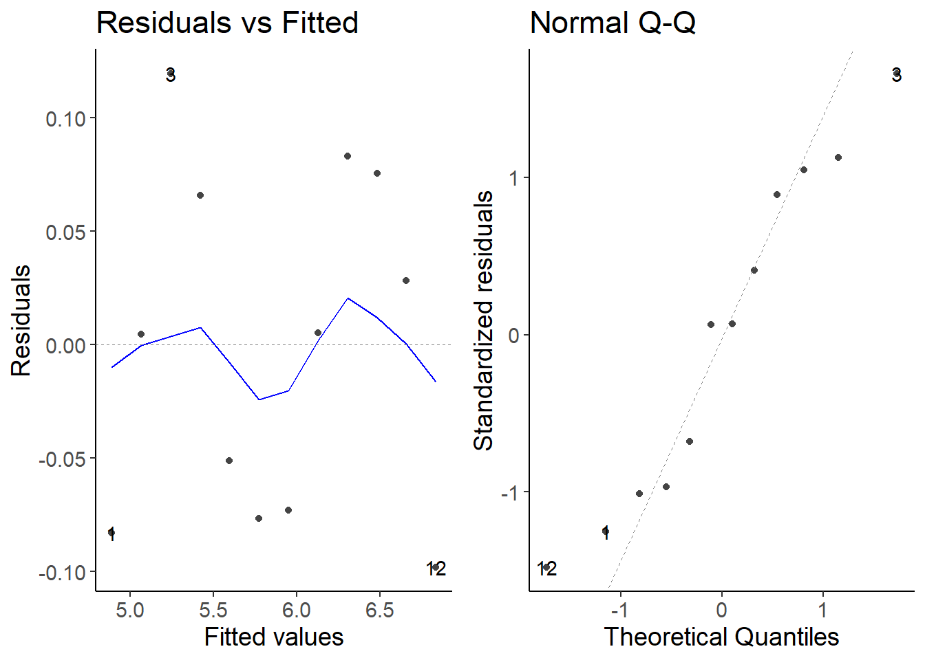
first_df <- mutate(first_df, cases7_pred = exp(predict(lm2)))

ggplot(first_df, aes(x = date, y = cases7)) +
    geom_point(size = 4) +
    geom_line(aes(y = cases7_pred),
              color = "red", linewidth = 1) +
    labs(x = "Date",
         y = "Reported cases of the last seven days",
title = "Reported covid cases in Berlin") 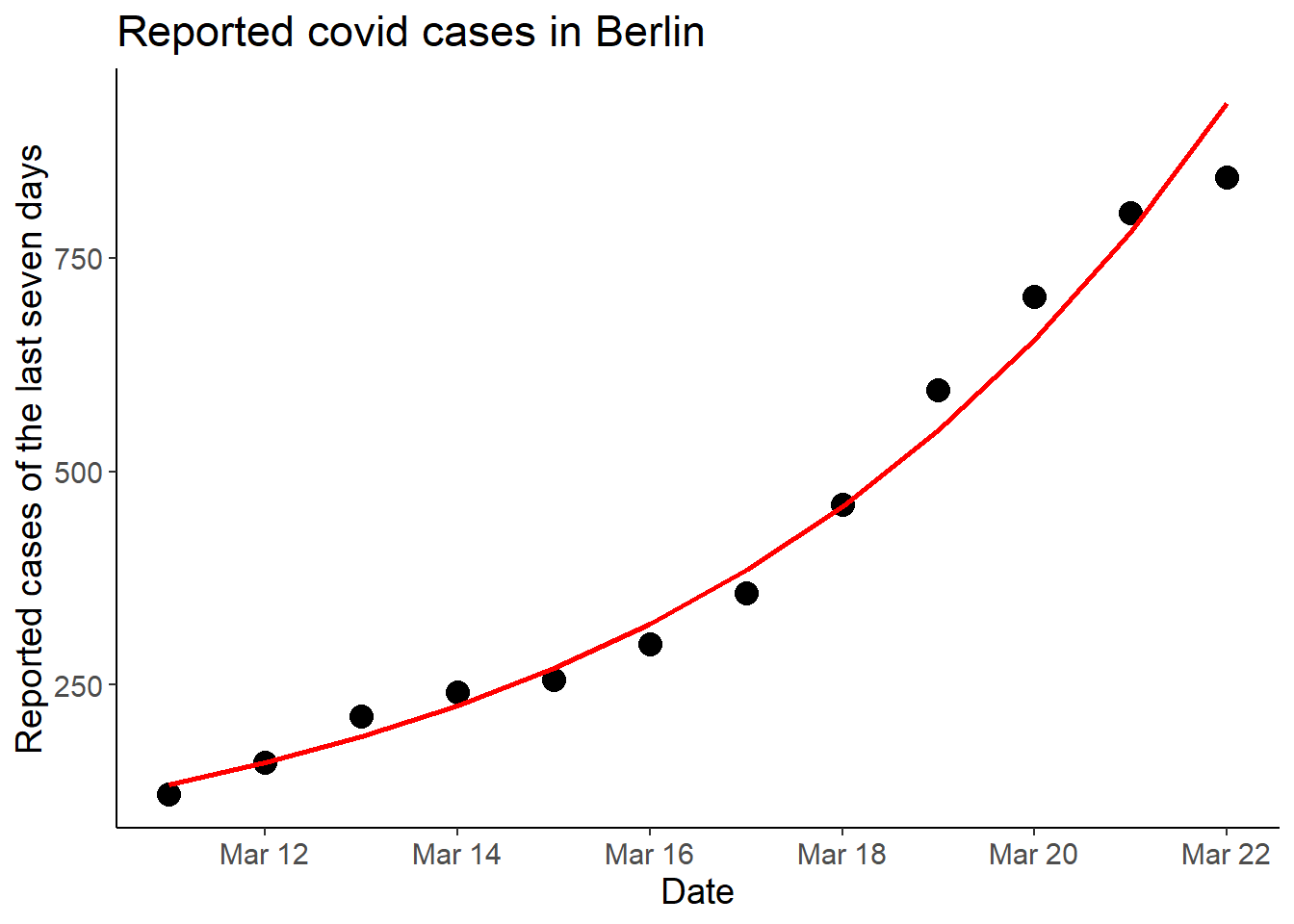
5 Fit model to second time period
second_df <- filter(df, date > "2021-10-15" & date < "2021-11-08" )

lm1_1 <- lm(cases7 ~ date, data = second_df)
autoplot(lm1_1, which = 1:2)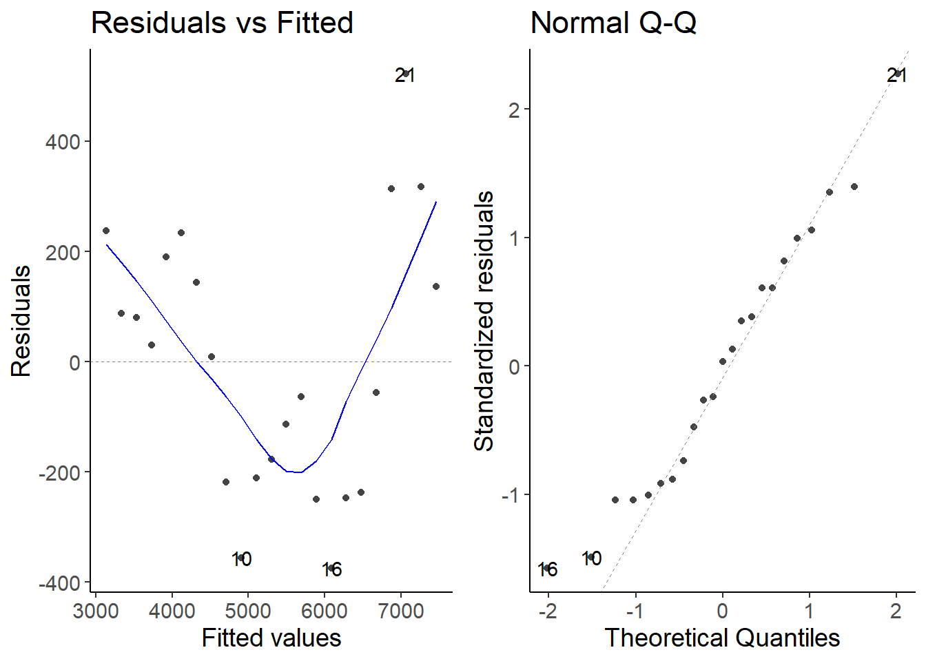
lm2_2 <- lm(log(cases7) ~ date, data = second_df)
autoplot(lm2_2, which = 1:2)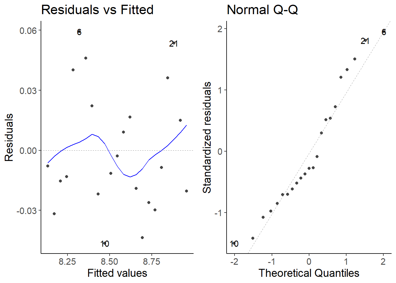
second_df <- mutate(second_df, cases7_pred = exp(predict(lm2_2)))

ggplot(second_df, aes(date, cases7)) +
    geom_point() +
    geom_line(aes(y = cases7_pred),
              color = "red", linewidth = 1) +
    labs(x = "Date",
         y = "Reported cases of the last seven days",
         title = "Reported covid cases in Berlin")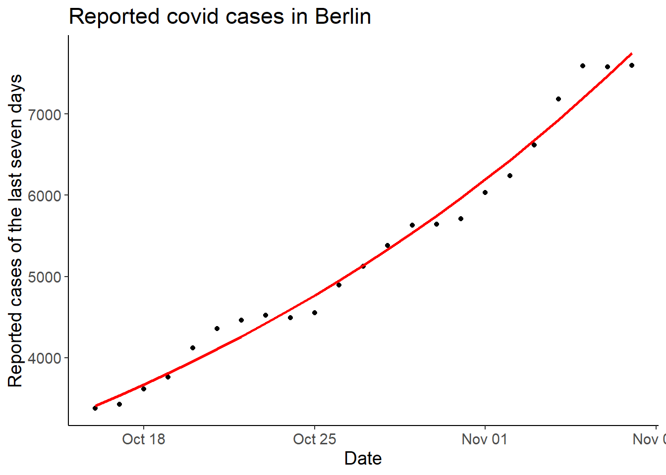
6 Everything together
library(readr)
library(dplyr)
library(ggplot2)
library(ggfortify)
library(tidyr)

theme_set(theme_classic())
theme_update(text = element_text(size = 14))

## read data and subset to Berlin
df <- read_csv("data/07_bl_infektionen.csv") %>%
    mutate(cases7 = bl_inz) %>%
    filter(bundesland == "Berlin") %>%
    rename(date = datum) %>%
    select(date, cases7)

## plot the number of cases over time
ggplot(df, aes(x = date, y = cases7)) +
    geom_line(size = 1) +
    labs(x = "Date",
            y = "Reported cases of the last seven days",
            title = "Reported covid cases in Berlin")

## fit model for first time period
first_df <- filter(df, date >= "2020-03-11" & date <= "2020-03-22" )

lm1 <- lm(cases7 ~ date, data = first_df)
autoplot(lm1, which = 1:2)

lm2 <- lm(log(cases7) ~ date, data = first_df)
autoplot(lm2, which = 1:2)

first_df <- mutate(first_df, cases7_pred = exp(predict(lm2)))

ggplot(first_df, aes(x = date, y = cases7)) +
    geom_point(size = 4) +
    geom_line(aes(y = cases7_pred),
              color = "red", linewidth = 1) +
    labs(x = "Date",
         y = "Reported cases of the last seven days",
         title = "Reported covid cases in Berlin")

## fit model for second time period
second_df <- filter(df, date > "2021-10-15" & date < "2021-11-08" )

lm1_1 <- lm(cases7 ~ date, data = second_df)
autoplot(lm1_1, which = 1:2)

lm2_2 <- lm(log(cases7) ~ date, data = second_df)
autoplot(lm2_2, which = 1:2)

second_df <- mutate(second_df, cases7_pred = exp(predict(lm2_2)))

ggplot(second_df, aes(date, cases7)) +
    geom_point() +
    geom_line(aes(y = cases7_pred),
              color = "red", linewidth = 1) +
    labs(x = "Date",
         y = "Reported cases of the last seven days",
         title = "Reported covid cases in Berlin")