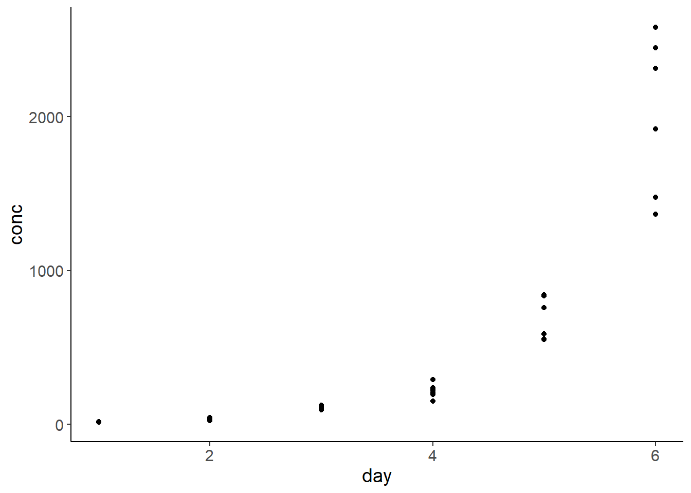
library(dplyr)library(readr)library(ggplot2)library(ggfortify)## theme for ggplottheme_set(theme_classic())theme_update(text =element_text(size =14))diatoms <-read_csv("data/07_diatoms.csv")# make a subset for species 1:diatoms1 <-filter(diatoms, species =="spec1"& pH =="low")# Plot the raw dataggplot(diatoms1, aes(day, conc)) +geom_point()
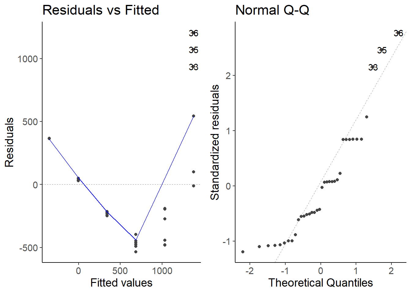
# Fit a model to the untransformed datamod1 <-lm(conc ~ day, data = diatoms1)# Check diagnostic plotsautoplot(mod1, which =1:2)
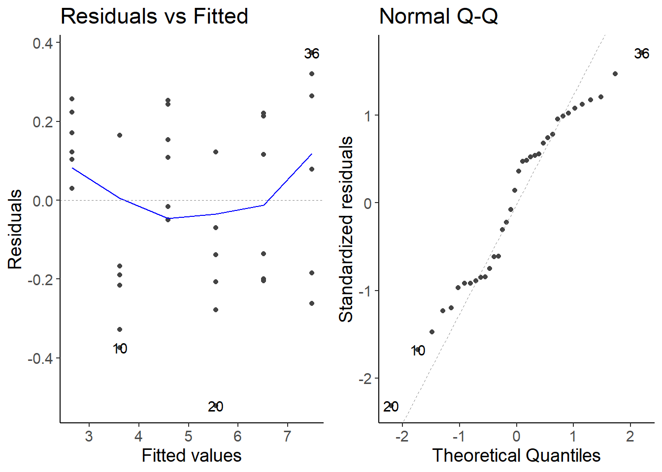
# Refit the model to transformed data# Try log transformmod2 <-lm(log(conc) ~ day, data = diatoms1)# Check diagnostic plots againautoplot(mod2, which =1:2)
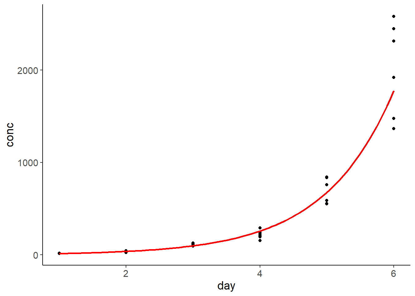
# Plot raw data again and add the model predictions # based on the transformed data# Create new and ordered time data and make predictionsdiatoms_pred <-tibble(day =seq(min(diatoms1$day),max(diatoms1$day),length =100)) %>%mutate(conc =exp(predict(mod2, newdata = .))) # Plot raw data and predictions againggplot(diatoms1, aes(day, conc)) +geom_point() +geom_line(data = diatoms_pred, color ="red", linewidth =1)
2 Everything as one script
library(dplyr)library(readr)library(ggplot2)library(ggfortify)## theme for ggplottheme_set(theme_classic())theme_update(text =element_text(size =14))diatoms <-read_csv("data/07_diatoms.csv")# make a subset for species 1:diatoms1 <-filter(diatoms, species =="spec1"& pH =="low")# Plot the raw dataggplot(diatoms1, aes(day, conc)) +geom_point() # Fit a model to the untransformed datamod1 <-lm(conc ~ day, data = diatoms1)# Check diagnostic plotsautoplot(mod1, which =1:2)# Refit the model to transformed data# Try log transformmod2 <-lm(log(conc) ~ day, data = diatoms1)# Check diagnostic plots againautoplot(mod2, which =1:2)# Plot raw data again and add the model predictions # based on the transformed data# Create new and ordered time data and make predictionsdiatoms_pred <-tibble(day =seq(min(diatoms1$day),max(diatoms1$day),length =100)) %>%mutate(conc =exp(predict(mod2, newdata = .))) # Plot raw data and predictions againggplot(diatoms1, aes(day, conc)) +geom_point() +geom_line(data = diatoms_pred, color ="red", linewidth =1)