## load packages
library(dplyr)
library(tidyr)
library(ggplot2)
library(ggfortify)
## theme for ggplot
theme_set(theme_classic())
theme_update(text = element_text(size = 14))
## create dataset
alpha <- 200
beta <- -3
sigma_val <- 10
nvalues <- 100
df <- tibble(
x = seq(0, 20, length = nvalues),
y = alpha + beta * x + rnorm(nvalues, mean = 0, sd = sigma_val))
## fit model
lm1 <- lm(y ~ x, data = df)
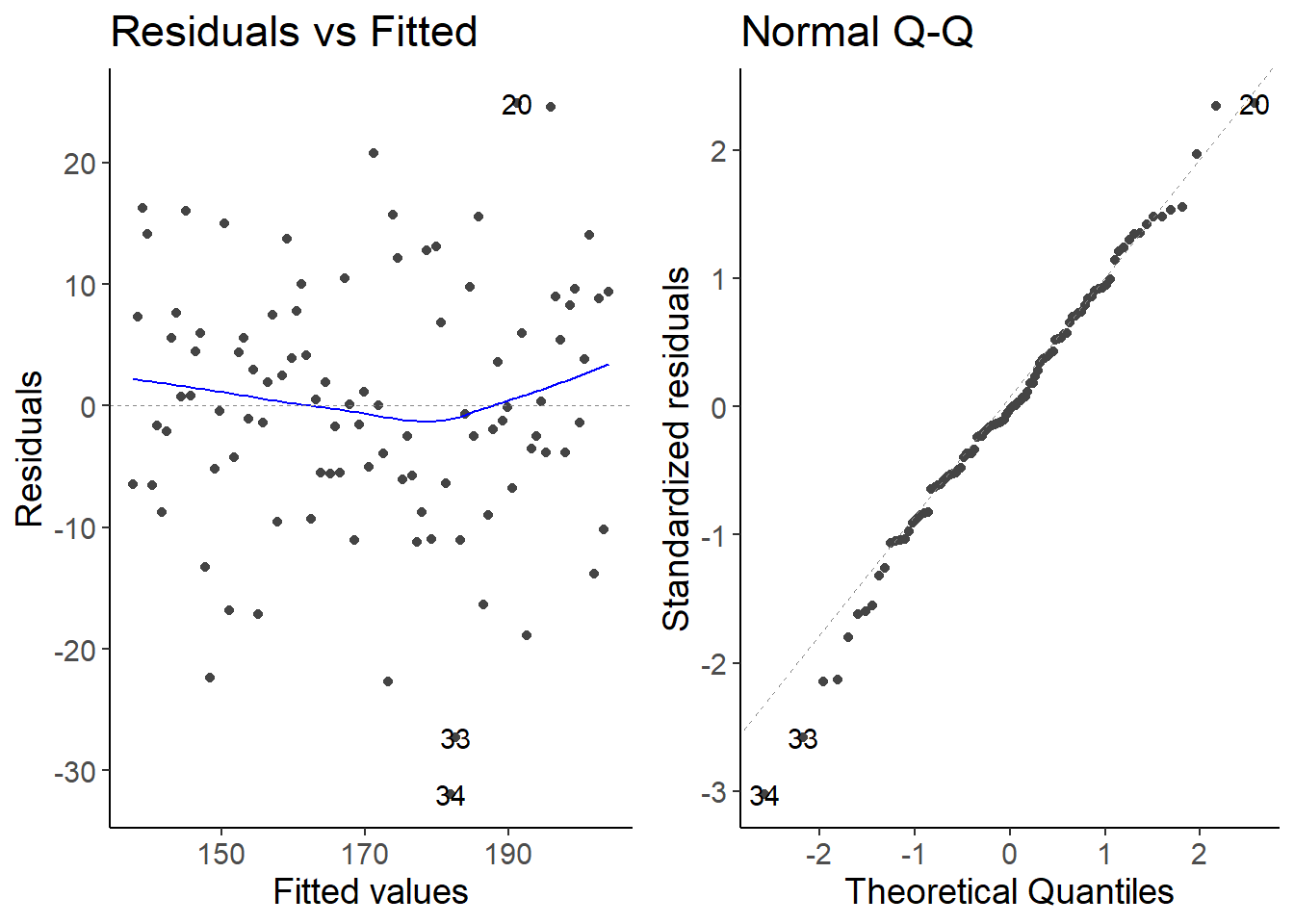
## check assumptions
autoplot(lm1, which = 1:2)
## check recovered parameters
lm1
sigma(lm1)
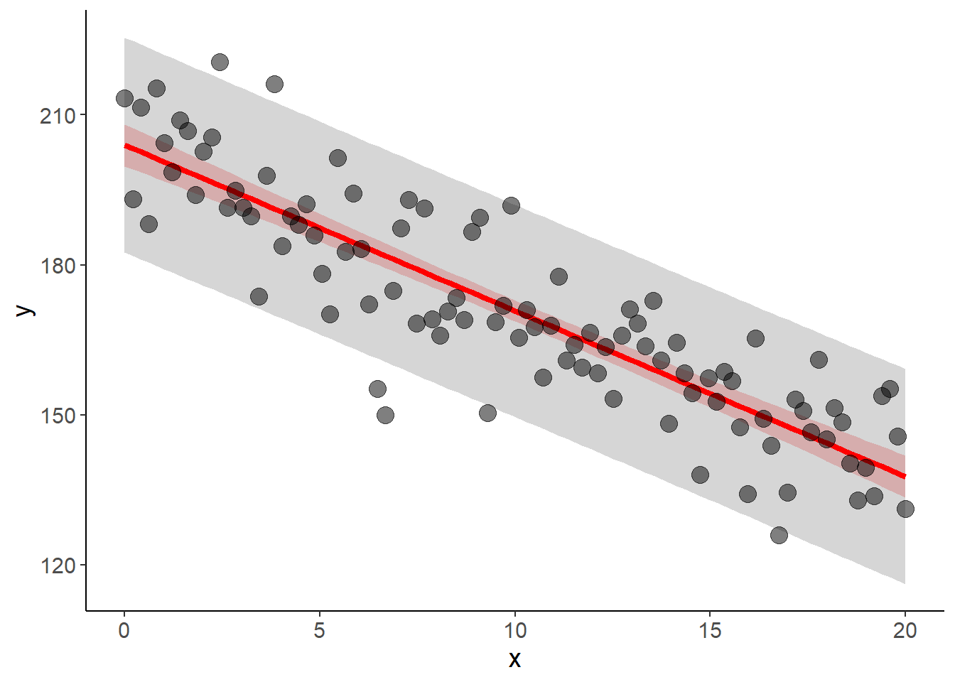
## plot predictions
df_pred <- tibble(x = seq(min(df$x), max(df$x), length = 100)) %>%
    bind_cols(predict(lm1, newdata = .,
                    interval = "confidence")) %>%
    rename(conf_low = lwr, conf_up = upr) %>%
    select(-fit) %>%
    bind_cols(predict(lm1, newdata = .,
                  interval = "prediction")) %>%
    rename(pred_low = lwr, pred_up = upr)

ggplot(df, aes(x, y)) +
    geom_ribbon(aes(y = fit, ymin = conf_low, ymax = conf_up),
                data = df_pred, fill = "red", alpha = 0.2) +
    geom_ribbon(aes(y = fit, ymin = pred_low, ymax = pred_up),
                data = df_pred,
                alpha = 0.2) +
    geom_line(aes(y = fit), data = df_pred,
              color = "red", linewidth = 1.5) +
    geom_point(size = 4, alpha = 0.5)