Script with output
## load packaes
library(dplyr)
library(readr)
library(ggplot2)
library(ggfortify)
## theme for ggplot
theme_set(theme_classic())
theme_update(text = element_text(size = 14))
## read datasets
df_ice <- read_csv("data/05_ice_cover.csv")
df_temp <- read_csv("data/05_ice_air_temp.csv")
## Mean air temperautre per year
df_yr_temp <- df_temp %>%
filter(year > 1884) %>%
summarise(temperature = mean(ave_air_temp_adjusted), .by = year)
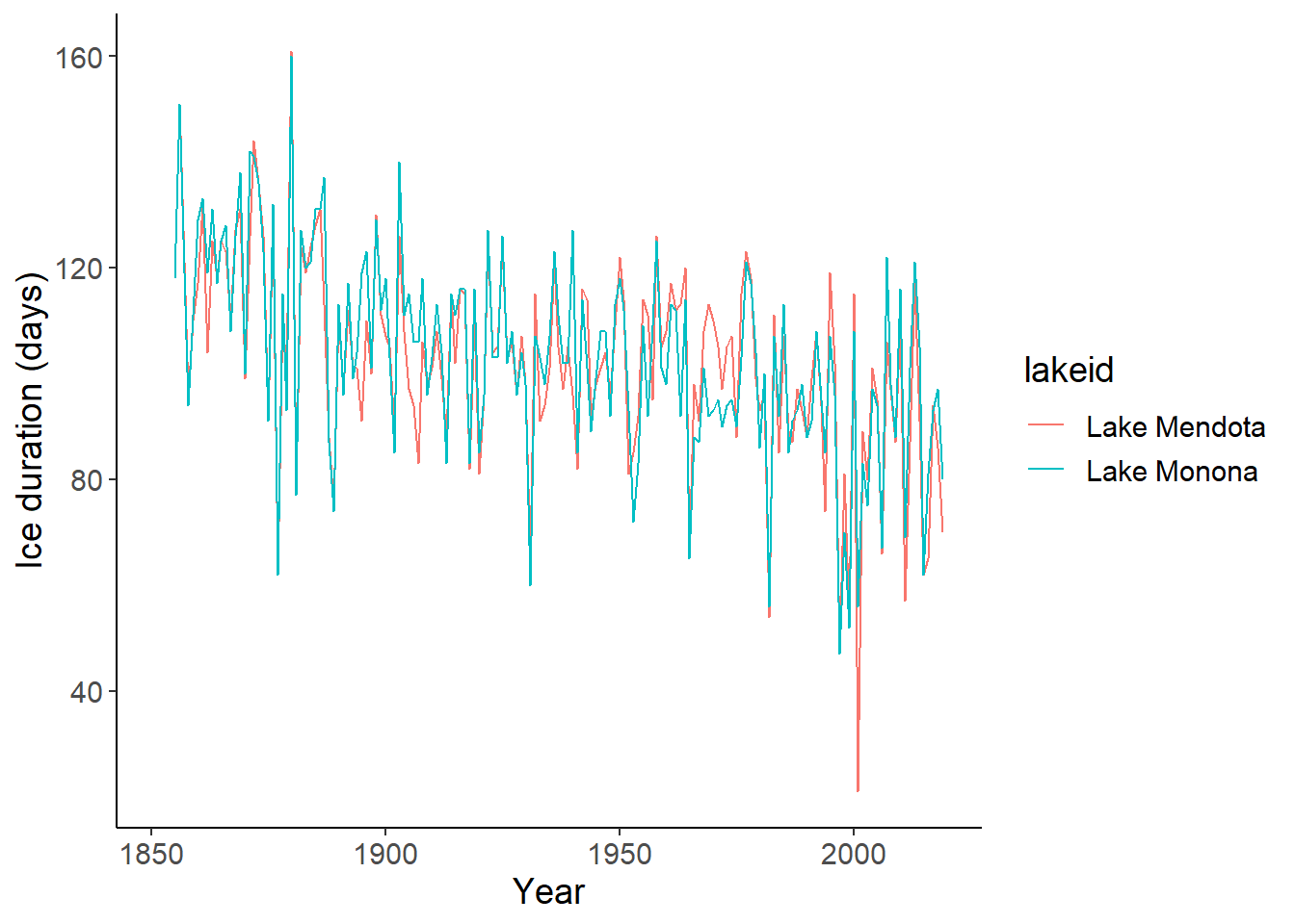
ggplot(df_ice, aes(year, ice_duration, color = lakeid)) +
geom_line() +
labs(x = "Year", y = "Ice duration (days)")
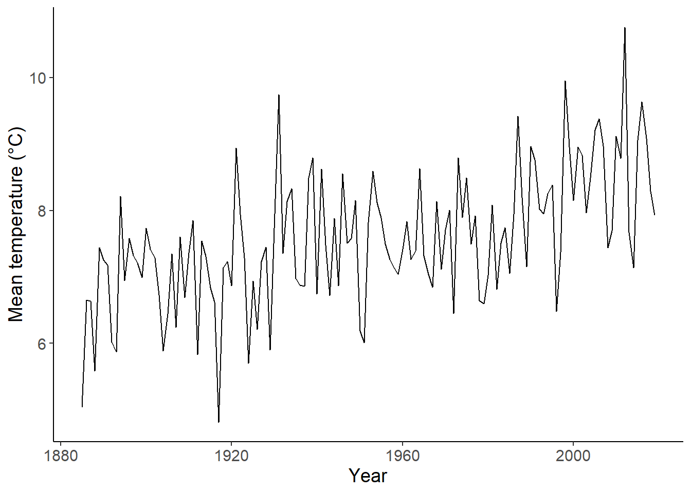
ggplot(df_yr_temp, aes(year, temperature)) +
    geom_line() +
    labs(x = "Year", y = "Mean temperature (°C)")
## calculate mean ice duration and join both dataset
df_ice_temp <- df_ice %>%
summarise(ice_duration = mean(ice_duration), .by = "year") %>%
inner_join(df_yr_temp, by = "year")
## fit linear model
lm1 <- lm(ice_duration ~ temperature, data = df_ice_temp)
## add predictions
df_ice_plot <- df_ice_temp %>%
bind_cols(predict(lm1, interval = "prediction", newdata = .))
## plot predictions
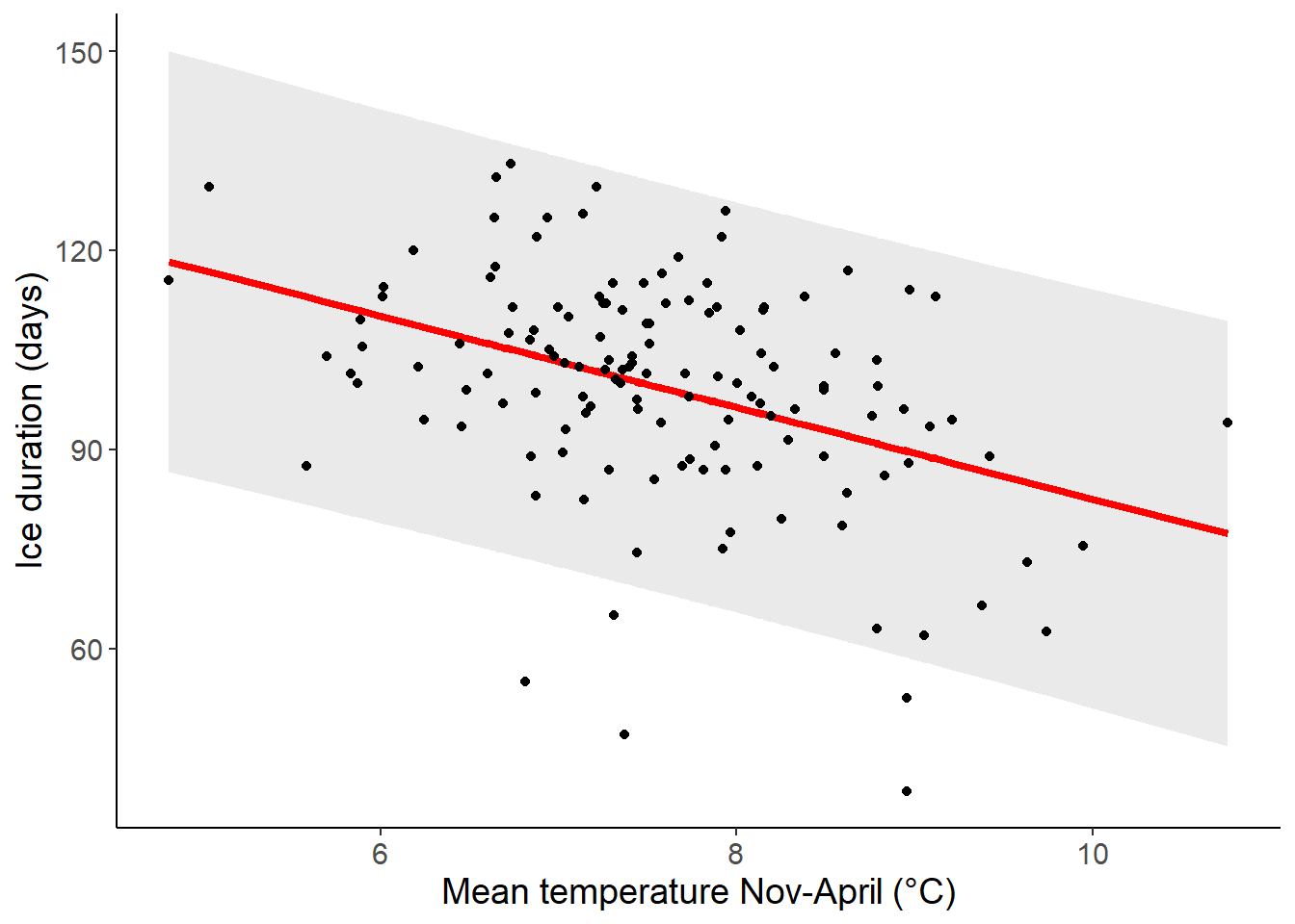
ggplot(df_ice_plot, aes(temperature, ice_duration)) +
geom_ribbon(aes(ymin = lwr, ymax = upr), alpha = 0.1) +
geom_line(aes(y = fit), linewidth = 1.5, color = "red") +
geom_point() +
labs(x = "Mean temperature Nov-April (°C)", y = "Ice duration (days)")
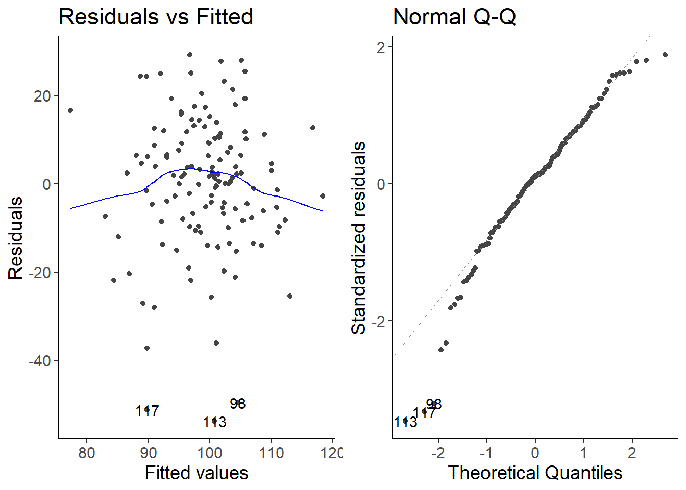
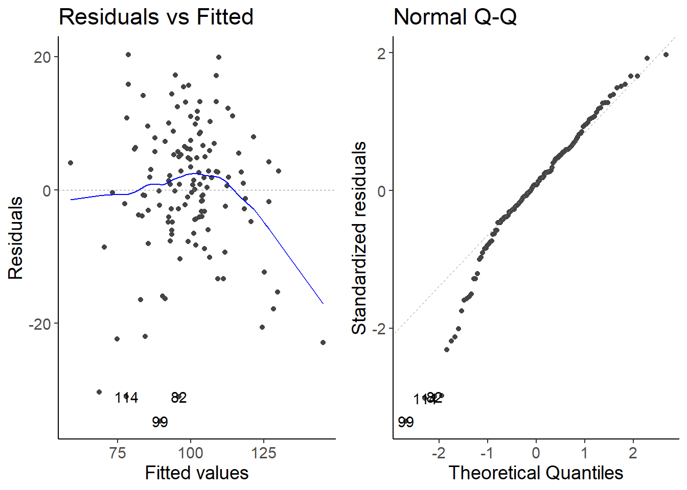
## check assumptions
autoplot(lm1, which = 1:2)
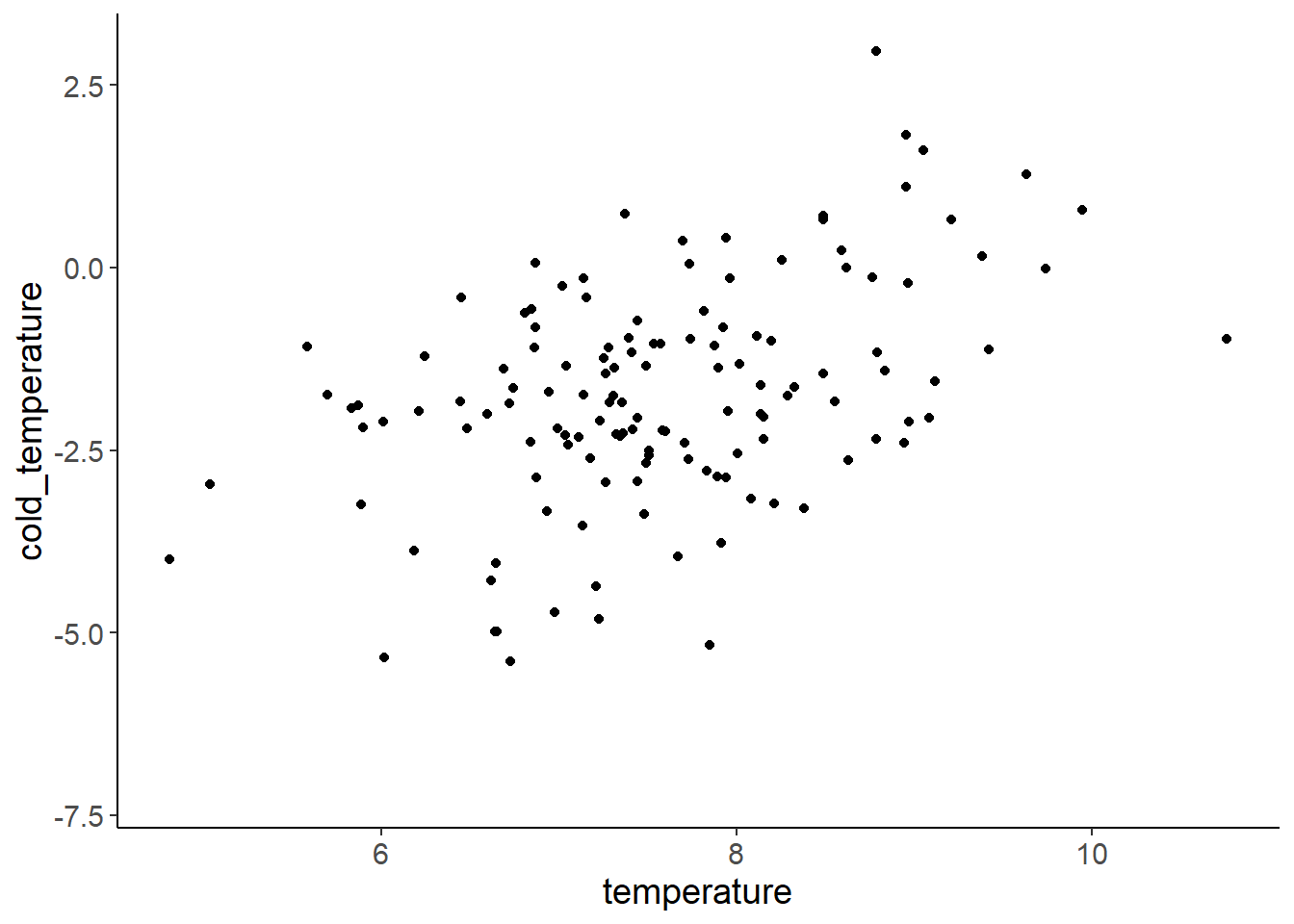
## bonus: mean temperature per hydrological year
# get month from date eihter by
# - lubridate::month(sampledate)
# - as.numeric(format(sampledate,"%m"))
df_hydroyr_temp <- df_temp %>%
    mutate(month = as.numeric(format(sampledate,"%m")),
           hydro_yr = ifelse(month < 10, year-1, year))  %>%
    filter(year > 1884) %>%
    filter(month %in% c(11:12,1:4)) %>%
    group_by(hydro_yr) %>%
    summarise(cold_temperature = mean(ave_air_temp_adjusted))

df_temp_join <- right_join(df_yr_temp, df_hydroyr_temp, by = c("year" = "hydro_yr"))

ggplot(df_temp_join, aes(temperature, cold_temperature)) +
  geom_point()
df_ice_hydro_temp <- df_ice %>%
summarise(ice_duration = mean(ice_duration), .by = "year") %>%
inner_join(df_hydroyr_temp, by = c("year" = "hydro_yr"))
## fit linear model
lm2 <- lm(ice_duration ~ cold_temperature, data = df_ice_hydro_temp)
## add predictions
df_ice_plot2 <- df_ice_hydro_temp %>%
bind_cols(predict(lm2, interval = "prediction", newdata = .))
## plot predictions
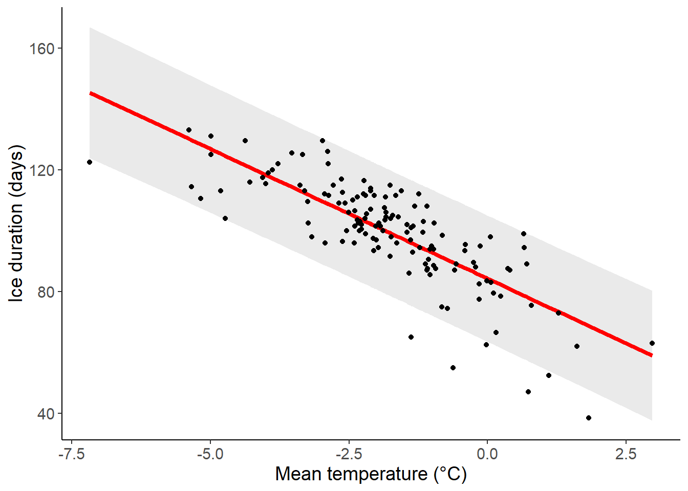
ggplot(df_ice_plot2, aes(cold_temperature, ice_duration)) +
geom_ribbon(aes(ymin = lwr, ymax = upr), alpha = 0.1) +
geom_line(aes(y = fit), linewidth = 1.5, color = "red") +
geom_point() +
labs(x = "Mean temperature (°C)", y = "Ice duration (days)")
## check assumptions
autoplot(lm2, which = 1:2)
Write down the equations
first model:
Call:
lm(formula = ice_duration ~ temperature, data = df_ice_temp)

Coefficients:
(Intercept)  temperature
     151.48        -6.89
\[
\begin{align}
\text{icecover} &= 151.48 -6.89 \cdot \text{temperature} + \epsilon \\
\epsilon &\sim N(0, 15.56) \\
\end{align}
\]
second model:
Call:
lm(formula = ice_duration ~ cold_temperature, data = df_ice_hydro_temp)

Coefficients:
     (Intercept)  cold_temperature
          84.293            -8.517
\[
\begin{align}
\text{icecover} &= 84.29 -8.52 \cdot \text{temperature} + \epsilon \\
\epsilon &\sim N(0, 10.40) \\
\end{align}
\]
Script for copy-pasting
## load packaes
library(dplyr)
library(readr)
library(ggplot2)
library(ggfortify)

## theme for ggplot
theme_set(theme_classic())
theme_update(text = element_text(size = 14))

## read datasets
df_ice <- read_csv("data/05_ice_cover.csv")
df_temp <- read_csv("data/05_ice_air_temp.csv")

## Mean air temperautre per year
df_yr_temp <- df_temp %>%
    filter(year > 1884) %>%
    summarise(temperature = mean(ave_air_temp_adjusted), .by = year)

ggplot(df_ice, aes(year, ice_duration, color = lakeid)) +
    geom_line() +
    labs(x = "Year", y = "Ice duration (days)")

ggplot(df_yr_temp, aes(year, temperature)) +
    geom_line() +
    labs(x = "Year", y = "Mean temperature (°C)")

## calculate mean ice duration and join both dataset
df_ice_temp <- df_ice %>%
  summarise(ice_duration = mean(ice_duration), .by = "year") %>%
  inner_join(df_yr_temp, by = "year")

## fit linear model
lm1 <- lm(ice_duration ~ temperature, data = df_ice_temp)

## add predictions
df_ice_plot <- df_ice_temp %>%
  bind_cols(predict(lm1, interval = "prediction", newdata = .))

## plot predictions
ggplot(df_ice_plot, aes(temperature, ice_duration)) +
    geom_ribbon(aes(ymin = lwr, ymax = upr), alpha = 0.1) +
    geom_line(aes(y = fit), linewidth = 1.5, color = "red") +
    geom_point() +
    labs(x = "Mean temperature Nov-April (°C)", y = "Ice duration (days)")

## check assumptions
autoplot(lm1, which = 1:2)

## bonus: mean temperature per hydrological year
# get month from date eihter by
# - lubridate::month(sampledate)
# - as.numeric(format(sampledate,"%m"))
df_hydroyr_temp <- df_temp %>%
    mutate(month = as.numeric(format(sampledate,"%m")),
           hydro_yr = ifelse(month < 10, year-1, year))  %>%
    filter(year > 1884) %>%
    filter(month %in% c(11:12,1:4)) %>%
    group_by(hydro_yr) %>%
    summarise(cold_temperature = mean(ave_air_temp_adjusted))

df_temp_join <- right_join(df_yr_temp, df_hydroyr_temp, by = c("year" = "hydro_yr"))

ggplot(df_temp_join, aes(temperature, cold_temperature)) +
  geom_point()

df_ice_hydro_temp <- df_ice %>%
  summarise(ice_duration = mean(ice_duration), .by = "year") %>%
  inner_join(df_hydroyr_temp, by = c("year" = "hydro_yr"))

## fit linear model
lm2 <- lm(ice_duration ~ cold_temperature, data = df_ice_hydro_temp)

## add predictions
df_ice_plot2 <- df_ice_hydro_temp %>%
  bind_cols(predict(lm2, interval = "prediction", newdata = .))

## plot predictions
ggplot(df_ice_plot2, aes(cold_temperature, ice_duration)) +
    geom_ribbon(aes(ymin = lwr, ymax = upr), alpha = 0.1) +
    geom_line(aes(y = fit), linewidth = 1.5, color = "red") +
    geom_point() +
    labs(x = "Mean temperature (°C)", y = "Ice duration (days)")

## check assumptions
autoplot(lm2, which = 1:2)