Solution to the maple exercise

## load packages
library(readr)
library(dplyr)
library(tidyr)
library(ggplot2)
library(ggfortify)

## theme for ggplot
theme_set(theme_classic())
theme_update(text = element_text(size = 14))

## read data
df_maples_prep <- read_csv("data/06_maples.csv")

## filter out missing values and rename factor levels
## and select columns
df_maples <- df_maples_prep %>%
  mutate(calcium_addition = factor(watershed, 
                                   levels = c("Reference", "W1"),
                                   labels = c("Control", "Ca addition"))) %>%
  select(stem_length, elevation, calcium_addition)
df_maples

# A tibble: 240 × 3
   stem_length elevation calcium_addition
         <dbl> <chr>     <fct>           
 1        86.9 Low       Control         
 2       114   Low       Control         
 3        83.5 Low       Control         
 4        68.1 Low       Control         
 5        72.1 Low       Control         
 6        77.7 Low       Control         
 7        85.5 Low       Control         
 8        81.6 Low       Control         
 9        92.9 Low       Control         
10        59.6 Low       Control         
# ℹ 230 more rows

## fit model without interaction
lm1 <- lm(stem_length ~ elevation + calcium_addition, data = df_maples)

## plot predictions
df_maples_pred <- expand_grid(
  elevation = c("Low", "Mid"),
  calcium_addition = c("Control", "Ca addition")) %>%
  bind_cols(predict(lm1, newdata = ., 
                    interval = "confidence")) %>%
  rename(conf_low = lwr, conf_up = upr) %>%
  select(-fit) %>%
  bind_cols(predict(lm1, newdata = ., 
                  interval = "prediction")) %>%
  rename(pred_low = lwr, pred_up = upr) 


ggplot(df_maples, aes(calcium_addition, stem_length, color = elevation)) +
  geom_point(size = 3, alpha = 0.3,
             position = position_jitterdodge(
                dodge.width = 1, jitter.width = 0.2, 
                jitter.height = 0.0)) +
  geom_pointrange(aes(y = fit, ymin = pred_low, ymax = pred_up),
                  data = df_maples_pred,
                  position = position_dodge(width = 1),
                  linewidth = 1, size = 0) +
  geom_pointrange(aes(y = fit, ymin = conf_low, ymax = conf_up),
                  data = df_maples_pred,
                  position = position_dodge(width = 1),
                  linewidth = 2, size = 0.8) +
  labs(x = "", y = "Stem length of seedlings (m)") 

## fit model with interaction
lm2 <- lm(stem_length ~ elevation * calcium_addition, data = df_maples)

1 Model equations and explanation

Without interaction:

lm1

Call:
lm(formula = stem_length ~ elevation + calcium_addition, data = df_maples)

Coefficients:
                (Intercept)                 elevationMid  
                     80.097                        1.776  
calcium_additionCa addition  
                      6.901  

sigma(lm1)

[1] 14.14383

The model is: \[ \begin{align} \text{stemlength} &= \cases { 80.10 + \epsilon, & \text{if low elevation and control} \\ 80.10 + 1.78 + \epsilon, & \text{if mid elevation and control} \\ 80.10 + 6.90 + \epsilon, & \text{if low elevation and calcium addition} \\ 80.10 + 1.78 + 6.90 + \epsilon, & \text{if mid elevation and calcium addition} \\ } \\ \epsilon &\sim \mathcal{N}(0, 14.14) \end{align} \]

With interaction:

lm2

Call:
lm(formula = stem_length ~ elevation * calcium_addition, data = df_maples)

Coefficients:
                             (Intercept)  
                                 80.1600  
                            elevationMid  
                                  1.6500  
             calcium_additionCa addition  
                                  6.7750  
elevationMid:calcium_additionCa addition  
                                  0.2517  

sigma(lm2)

[1] 14.17362

\[ \begin{align} \text{stemlength} &= \cases { 80.16 + \epsilon, & \text{if low elevation and control} \\ 80.16 + 1.65 + \epsilon, & \text{if mid elevation and control} \\ 80.16 + 6.78 + \epsilon, & \text{if low elevation and calcium addition} \\ 80.16 + 1.65 + 6.78 + 0.25 + \epsilon, & \text{if mid elevation and calcium addition} \\ } \\ \epsilon &\sim \mathcal{N}(0, 14.17) \end{align} \]

Which model is better?

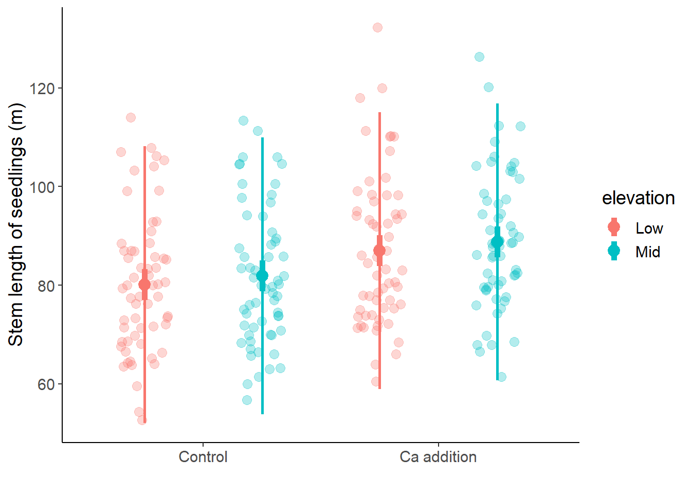
The estimate of the interaction is quite low. The adjusted R² is lower for the second model. Therefore, if you want to make good predictions it is better to use the first model.