Solution to the penguins exercise

1 Load packages

library(dplyr)
library(readr)
library(ggplot2)
library(ggfortify)

## theme for ggplot
theme_set(theme_classic())
theme_update(text = element_text(size = 14))

2 Load data and fit model

df_penguins <- read_csv("data/05_penguins.csv") 
lm1 <- lm(bill_length_mm ~ species, data = df_penguins)
summary(lm1)


Call:
lm(formula = bill_length_mm ~ species, data = df_penguins)

Residuals:
    Min      1Q  Median      3Q     Max 
-7.9338 -2.2049  0.0086  2.0662 12.0951 

Coefficients:
                 Estimate Std. Error t value Pr(>|t|)    
(Intercept)       38.7914     0.2409  161.05   <2e-16 ***
speciesChinstrap  10.0424     0.4323   23.23   <2e-16 ***
speciesGentoo      8.7135     0.3595   24.24   <2e-16 ***
---
Signif. codes:  0 '***' 0.001 '**' 0.01 '*' 0.05 '.' 0.1 ' ' 1

Residual standard error: 2.96 on 339 degrees of freedom
  (2 observations deleted due to missingness)
Multiple R-squared:  0.7078,    Adjusted R-squared:  0.7061 
F-statistic: 410.6 on 2 and 339 DF,  p-value: < 2.2e-16

Model equation:

\[ \begin{align} \text{billlength} &= \cases{ 38.8 + \epsilon, & \text{ if Adelie} \\ 38.8 + 10 + \epsilon, & \text{ if Chinstrap} \\ 38.8 + 8.7 + \epsilon, & \text{ if Gentoo} \\ } \\ \epsilon &\sim \mathcal{N}(0, 3) \end{align} \]

3 Check assumptions

autoplot(lm1, which = 1:2)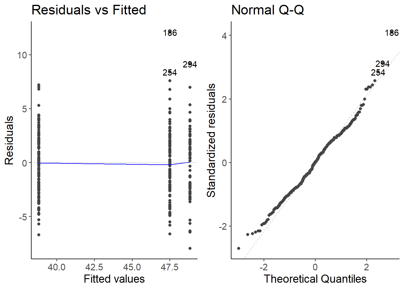

4 Make predictions

df_penguins_pred <- tibble(species = unique(df_penguins$species)) %>%
    bind_cols(predict(lm1, newdata = ., 
                      interval = "prediction", level = 0.95)) %>%
    rename(bill_length_mm = fit)

5 Different ways to visualize the data

boxplot + jitterplot

ggplot(df_penguins, aes(species, bill_length_mm)) +
    geom_boxplot(outlier.shape = NA) + 
    geom_jitter(width = 0.3, height = 0, alpha = 0.5, size = 2) +
    geom_pointrange(aes(ymin = lwr, ymax = upr), data = df_penguins_pred, 
                    color = "red", linewidth = 1.5, size = 2, alpha = 0.6) +
    labs(y = "Bill length [mm]")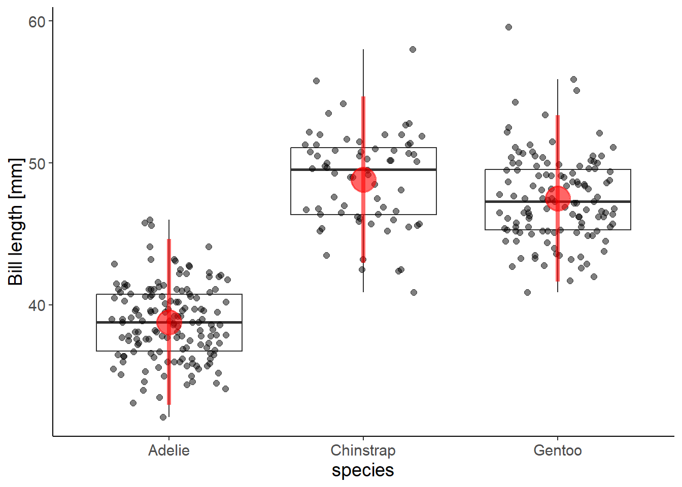

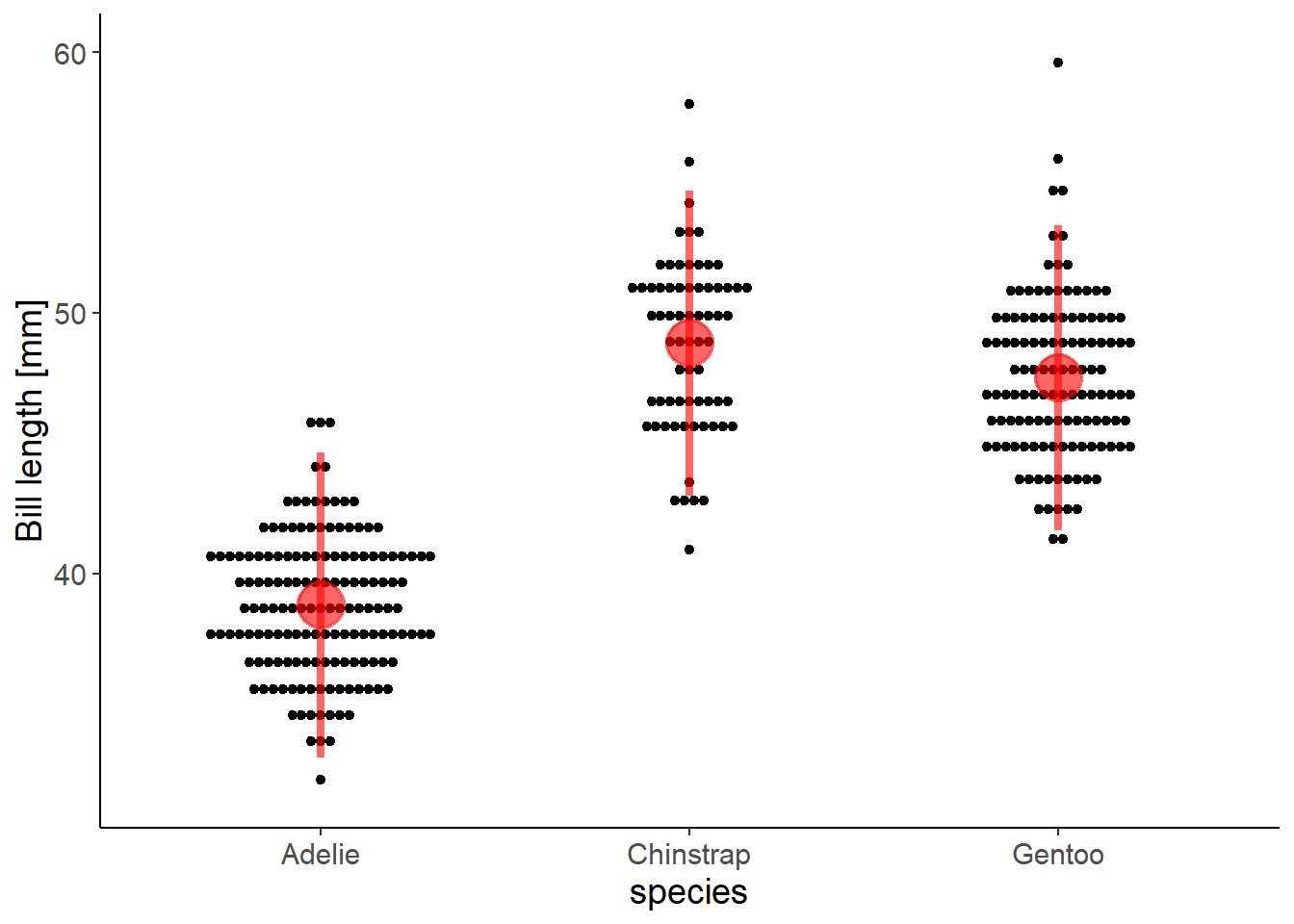
dot plot (similar to a histogram)

ggplot(df_penguins, aes(species, bill_length_mm)) +
    geom_dotplot(binaxis = "y", dotsize = 0.4, stackdir = "center") +
    geom_pointrange(aes(ymin = lwr, ymax = upr), data = df_penguins_pred, 
                    color = "red", linewidth = 1.5, size = 2, alpha = 0.6) +
    labs(y = "Bill length [mm]")