Solution to influence of plant species richness on productivity exercise

1 Load packages

library(readr)
library(dplyr)
library(ggplot2)
library(ggfortify)

## theme for ggplot
theme_set(theme_classic())
theme_update(text = element_text(size = 14))

1.1 Read and plot data

df_prod <- read_csv("data/05_productivity.csv")
df_prod_sub <- filter(df_prod, site == "site1")

ggplot(df_prod_sub, aes(richness, productivity)) +
  geom_point() +
  labs(x = "Species richness", y = "Productivity g/(m²yr)")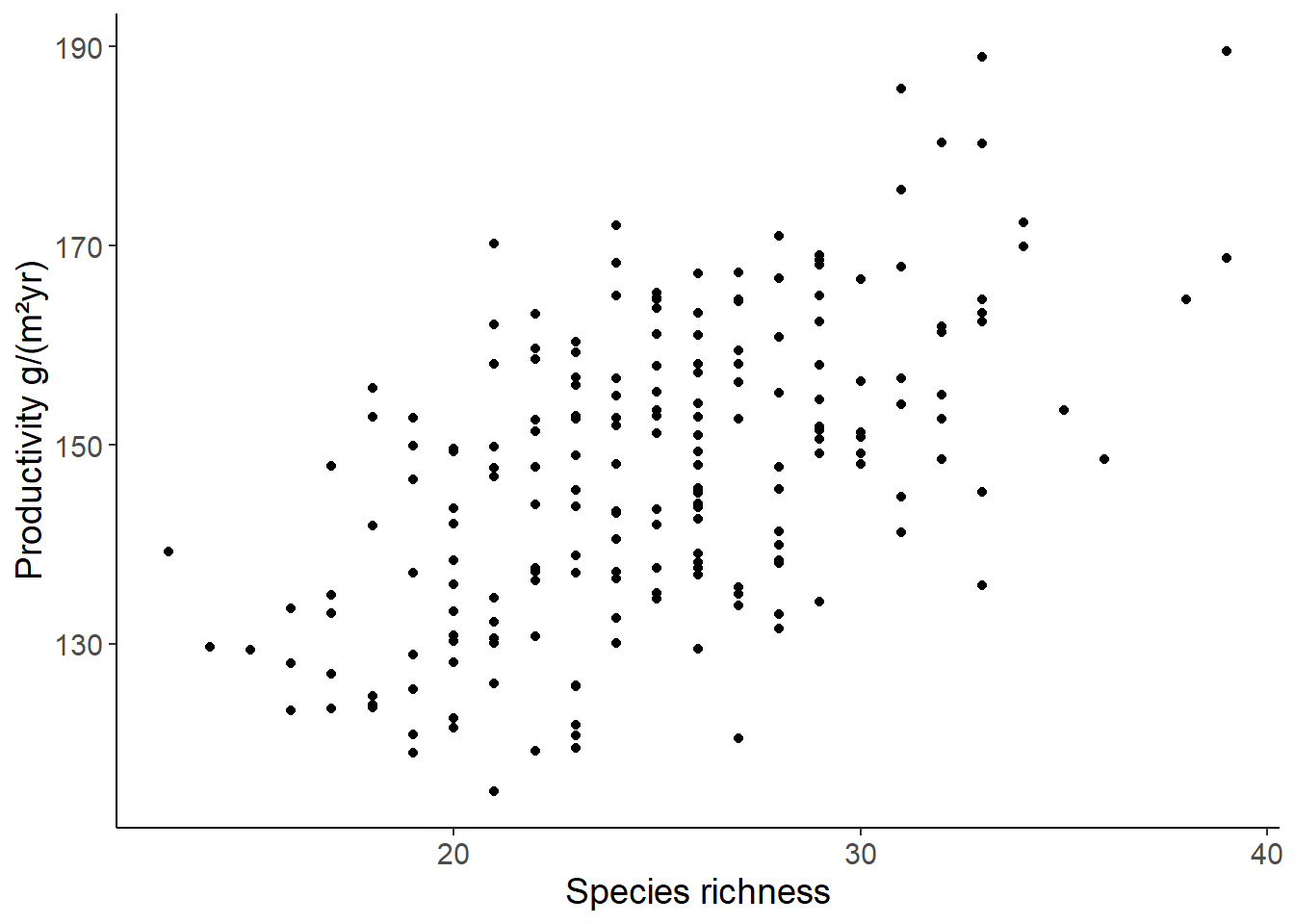

2 Fit model and plot predictions

lm1 <- lm(productivity ~ richness, data = df_prod_sub)  

## use abline to plot the regression line
b <- coef(lm1)[1]
m <- coef(lm1)[2]
ggplot(df_prod_sub, aes(richness, productivity)) +
  geom_point() +
  geom_abline(intercept = b, slope = m,
              color = "red", linewidth = 1) +
  labs(x = "Species richness", y = "Productivity g/(m²yr)")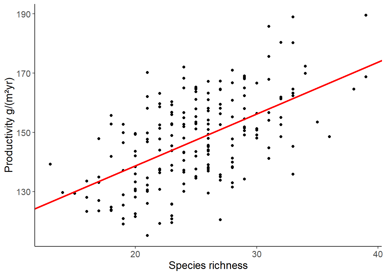

## use predict to add the predicted values to the data table
## if we do not specify a new data set, the model is used to predict the values of the data set that was used to fit the model
df_prod_sub <- mutate(df_prod_sub, productivity_pred = predict(lm1))  

ggplot(df_prod_sub, aes(richness, productivity)) +
    geom_point() +
    geom_line(aes(y = productivity_pred), color = "red", size = 1) +
    labs(x = "Species richness", y = "Productivity g/(m²yr)")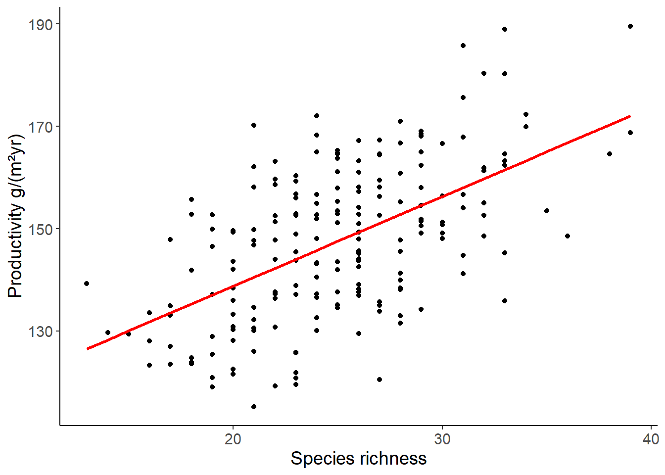

## here we specify a new data set to predict the values
## if you want to create many values, use seq(start, stop, length = n)
## or if you have several predictor variables, use expand_grid() 
## with seq() for each variable
df_prod_pred <- tibble(richness = c(20, 30)) %>%
  mutate(productivity = predict(lm1, newdata = .))

ggplot(df_prod_sub, aes(richness, productivity)) +
    geom_point() +
    geom_line(data = df_prod_pred, color = "red", size = 1) +
    labs(x = "Species richness", y = "Productivity g/(m²yr)")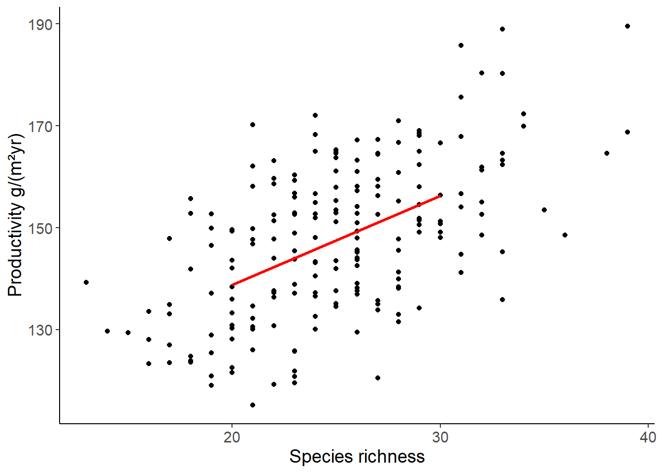

2.1 How to read the output of the model and centering the predictor variable

summary(lm1)

Call:
lm(formula = productivity ~ richness, data = df_prod_sub)

Residuals:
     Min       1Q   Median       3Q      Max 
-30.5474  -9.3837  -0.3206   9.3048  29.6546 

Coefficients:
            Estimate Std. Error t value Pr(>|t|)    
(Intercept) 103.7883     4.6444  22.347   <2e-16 ***
richness      1.7503     0.1826   9.583   <2e-16 ***
---
Signif. codes:  0 '***' 0.001 '**' 0.01 '*' 0.05 '.' 0.1 ' ' 1

Residual standard error: 12.49 on 198 degrees of freedom
Multiple R-squared:  0.3169,    Adjusted R-squared:  0.3134 
F-statistic: 91.84 on 1 and 198 DF,  p-value: < 2.2e-16

Equation of the first model: \[ \begin{align} \text{productivity} &= 103.79 + 1.75 \cdot \text{richness} + \epsilon \\ \epsilon &\sim \mathcal{N}(0, 12.49) \end{align} \]

When you add one species, the model predicts that the productivity increases by 1.75 g/(m²yr). The intercept is the predicted productivity when richness is zero. This is not a meaningful value in this case, because you cannot have a productivity if no plant species are present at all.

If you want to have a meaningful intercept, you can center the predictor variable. This means that you subtract the mean from each value. The mean of the centered variable is then zero. The intercept is then the predicted value when the predictor is at its mean value:

mutate(df_prod_sub, c_richness = richness - mean(richness)) %>%
  lm(productivity ~ c_richness, data = .) %>%
  summary()

Call:
lm(formula = productivity ~ c_richness, data = .)

Residuals:
     Min       1Q   Median       3Q      Max 
-30.5474  -9.3837  -0.3206   9.3048  29.6546 

Coefficients:
            Estimate Std. Error t value Pr(>|t|)    
(Intercept) 147.4855     0.8830 167.025   <2e-16 ***
c_richness    1.7503     0.1826   9.583   <2e-16 ***
---
Signif. codes:  0 '***' 0.001 '**' 0.01 '*' 0.05 '.' 0.1 ' ' 1

Residual standard error: 12.49 on 198 degrees of freedom
Multiple R-squared:  0.3169,    Adjusted R-squared:  0.3134 
F-statistic: 91.84 on 1 and 198 DF,  p-value: < 2.2e-16

R²:

The R² of the model is 0.32, and the adjusted R² 0.31. That means the independent variable(s) can explain 32 % (adjusted 31 %) of the variance of the dependent variable. The adjusted R² is always smaller than the R², and it is used to compare models with different numbers of predictor variables.

2.2 Check the model assumptions

autoplot(lm1, which = 1:2)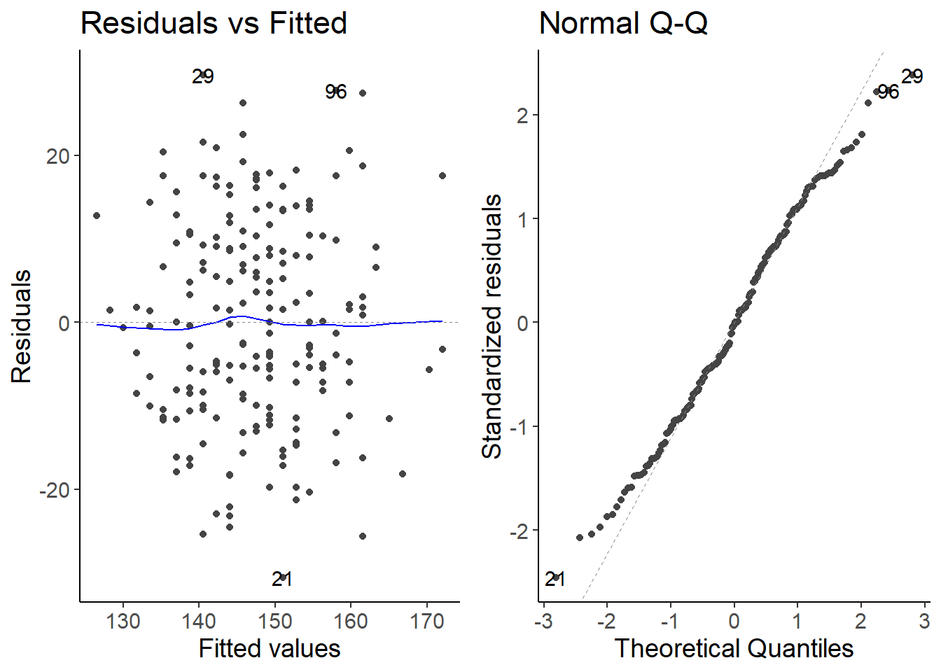

2.3 Fit a model for the second site

df_prod_sub2 <- filter(df_prod, site == "site2")

lm2 <- lm(productivity ~ richness, data = df_prod_sub2)

autoplot(lm2, which = 1:2)

The variance of the residuals is increasing with higher values of the predictor variable. This is called heteroscedasticity. We can transform the response variable or use a generalized linear model with a different error distribution.