Solution for binomial GLM with binary data

1 Solution with R output

First, we prepare the session by loading the necessary packages and adjust the theme for ggplot. Adjusting the theme is of course optional and not necessary.

library(readr)
library(ggplot2)
library(dplyr)
library(tidyr)

## theme for ggplot
theme_set(theme_classic())
theme_update(text = element_text(size = 14))

Now, we load the data and create a plot with the presence/absence of Odonates at the y-axis and the measure of bromeliad size at the x-axis.

# Read the data
bromeliads <- read_csv("data/08_bromeliads.csv")

ggplot(bromeliads, aes(x = logmaxvolume, y = Odonatepresence)) +
  geom_point()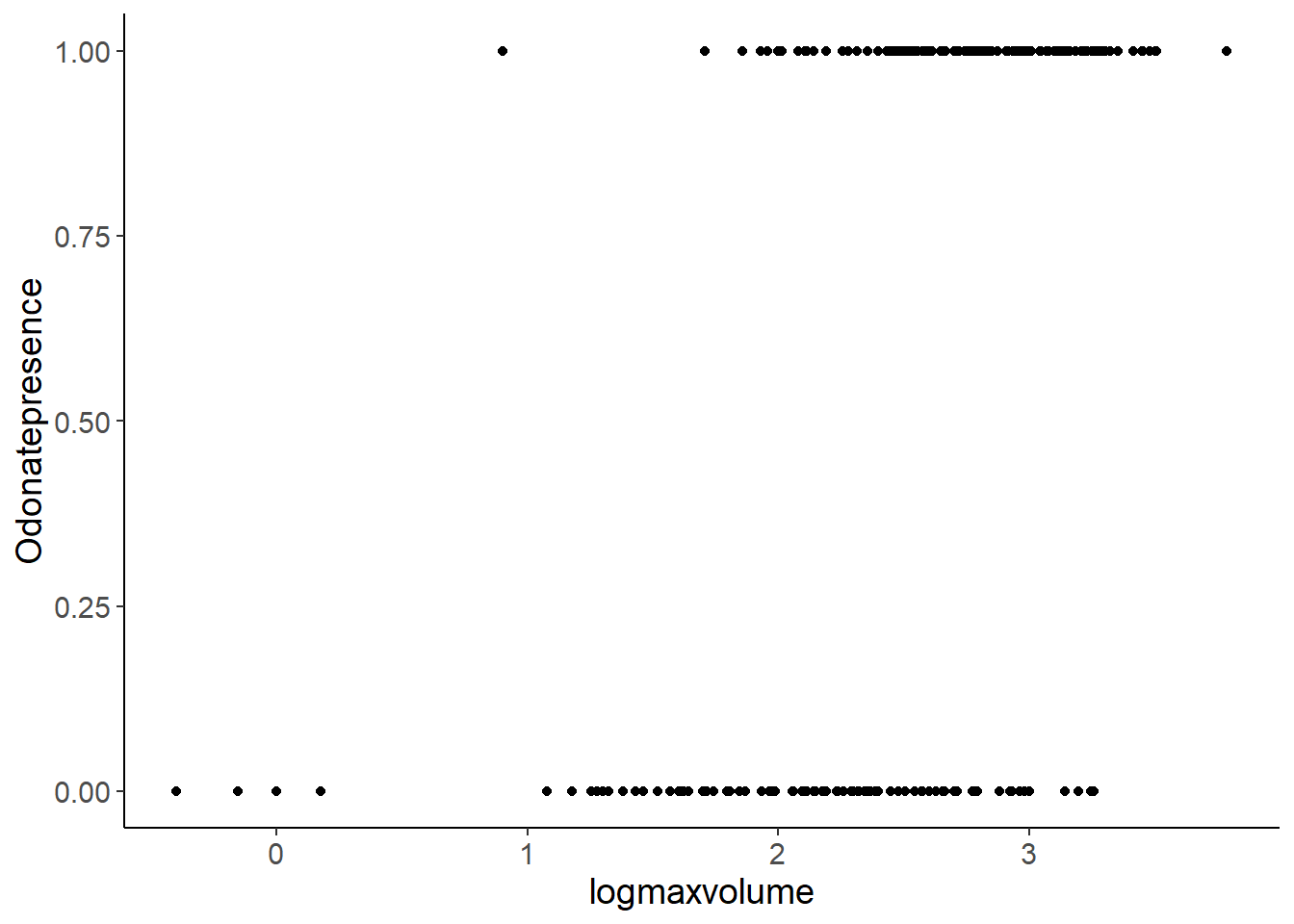

This looks a bit weird, because of the binary data, which only includes 0 (Odonates absent) and 1 (Odonates present) values. Jittering in vertical direction helps a bit for the visualisation.

ggplot(bromeliads, aes(x = logmaxvolume, y = Odonatepresence)) +
  geom_jitter(height = 0.1, width = 0, size = 2, alpha = 0.5)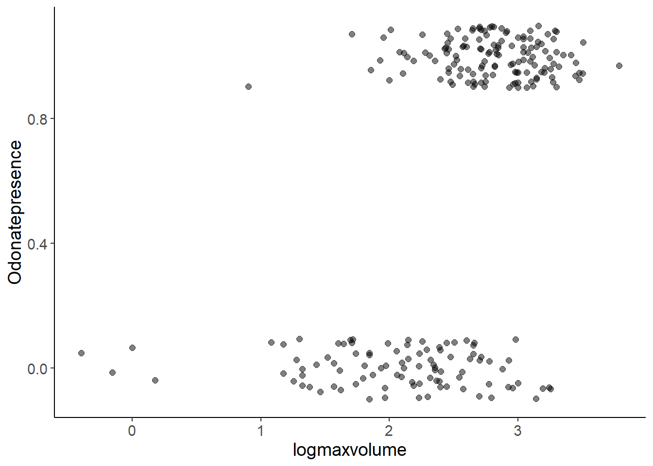 

For binary data, we use a GLM with Binomial error distribution - and logit-link by default. We fit this model and test the effect of bromeliad volume on the presence/absence of Odonates with a Likelihood-Ratio-Test using the R function drop1().

model1 <- glm(Odonatepresence ~ logmaxvolume,
              family = binomial(link = "logit"),
              data = bromeliads)
drop1(model1, test = "Chi")

Single term deletions

Model:
Odonatepresence ~ logmaxvolume
             Df Deviance    AIC    LRT  Pr(>Chi)    
<none>            226.57 230.57                     
logmaxvolume  1   316.07 318.07 89.504 < 2.2e-16 ***
---
Signif. codes:  0 '***' 0.001 '**' 0.01 '*' 0.05 '.' 0.1 ' ' 1

The test tells us that there is a clear statistical association between bromeliad size and Odonate presence/absence, but it does not tell us about the direction of the effect. For this, we can check the summary of the model:

summary(model1)

Call:
glm(formula = Odonatepresence ~ logmaxvolume, family = binomial(link = "logit"), 
    data = bromeliads)

Coefficients:
             Estimate Std. Error z value Pr(>|z|)    
(Intercept)   -6.5292     0.9876  -6.611 3.81e-11 ***
logmaxvolume   2.7594     0.3870   7.130 1.00e-12 ***
---
Signif. codes:  0 '***' 0.001 '**' 0.01 '*' 0.05 '.' 0.1 ' ' 1

(Dispersion parameter for binomial family taken to be 1)

    Null deviance: 316.07  on 233  degrees of freedom
Residual deviance: 226.57  on 232  degrees of freedom
AIC: 230.57

Number of Fisher Scoring iterations: 5

Here, the positive value of the slope estimate for logmaxvolume (2.76) indicates that the probability of Odonate presence increases with size. In other words: the bigger the bromeliad the more likely is it that we find Odonates.

Finally, we add the predicted curve to the plot with the data in the usual way:

1. Create new values for the independent variable (logmaxvolume).
2. Add predictions. Note the type = "response" argument.
3. Plot data and prediction.

min_vol <- min(bromeliads$logmaxvolume)
max_vol <- max(bromeliads$logmaxvolume)

odonate_pred <- tibble(logmaxvolume = seq(min_vol,
                                          max_vol,
                                          length = 200))
odonate_pred$pred <- predict(model1, newdata = odonate_pred,
                             type = "response")

ggplot(bromeliads, aes(x = logmaxvolume, y = Odonatepresence)) +
  geom_jitter(height = 0.1, width = 0, size = 2, alpha = 0.5)  +
  geom_line(aes(logmaxvolume, pred), data = odonate_pred,
            color = "red")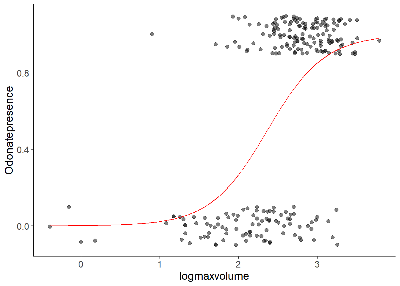

What does the red line show? It does not show the presence or absence of Odonates, because this can only be 0 or 1, but it shows the probability of Odonate presence depending on logmaxvolume. The sigmoidal shape is a consequence of the inverse logit-link function. See slide 11.

1.1 Extra

We now add the site as potential explanatory variable and fit a model that includes an interaction between logmaxvolume and site. This means the model allows different relationships between logmaxvolume and Odonate presence/absence in each site.

model2 <- glm(Odonatepresence ~ logmaxvolume * site,
                  family = binomial, data = bromeliads)
drop1(model2, test = "Chi")

Single term deletions

Model:
Odonatepresence ~ logmaxvolume * site
                  Df Deviance    AIC    LRT Pr(>Chi)    
<none>                 192.18 208.18                    
logmaxvolume:site  3   219.27 229.27 27.089 5.64e-06 ***
---
Signif. codes:  0 '***' 0.001 '**' 0.01 '*' 0.05 '.' 0.1 ' ' 1

We get a warning and a highly significant interaction, which is strange. To understand this better, we look first at the summary and second at the predictions.

summary(model2)

Call:
glm(formula = Odonatepresence ~ logmaxvolume * site, family = binomial, 
    data = bromeliads)

Coefficients:
                              Estimate Std. Error z value Pr(>|z|)   
(Intercept)                    -2.3998     1.3952  -1.720  0.08541 . 
logmaxvolume                    1.3629     0.5588   2.439  0.01474 * 
siteMacae                     -15.0410     5.0498  -2.979  0.00290 **
sitePicinguaba              -1387.3681 91853.4151  -0.015  0.98795   
sitePitilla                    -6.2907     2.1950  -2.866  0.00416 **
logmaxvolume:siteMacae          5.0983     1.8170   2.806  0.00502 **
logmaxvolume:sitePicinguaba   571.3793 37840.3201   0.015  0.98795   
logmaxvolume:sitePitilla        2.3405     0.8972   2.609  0.00909 **
---
Signif. codes:  0 '***' 0.001 '**' 0.01 '*' 0.05 '.' 0.1 ' ' 1

(Dispersion parameter for binomial family taken to be 1)

    Null deviance: 316.07  on 233  degrees of freedom
Residual deviance: 192.18  on 226  degrees of freedom
AIC: 208.18

Number of Fisher Scoring iterations: 19

We can see that something is strange about the site Picinguaba. Its parameter estimate for intercept and slope are really big and at the same time completely uncertain. Please note the extremely high Standard Errors in the second column (Std. Error) of the coefficient table.

The best way to understand this is looking at the predictions and the data. We now have to explanatory variables, so we use expand_grid() to generate all combinations of site and logmaxvolume.

pred_dat <- expand_grid(logmaxvolume = seq(min_vol,
                                           max_vol,
                                          length = 200),
                        site = unique(bromeliads$site))
pred_dat$pred_prob <- predict(model2, newdata = pred_dat, type = "response")

ggplot(bromeliads, aes(x = logmaxvolume, y = Odonatepresence, color = site)) +
  geom_jitter(height = 0.1, width = 0, size = 2, alpha = 0.5) +
  geom_line(aes(logmaxvolume, pred_prob), data = pred_dat)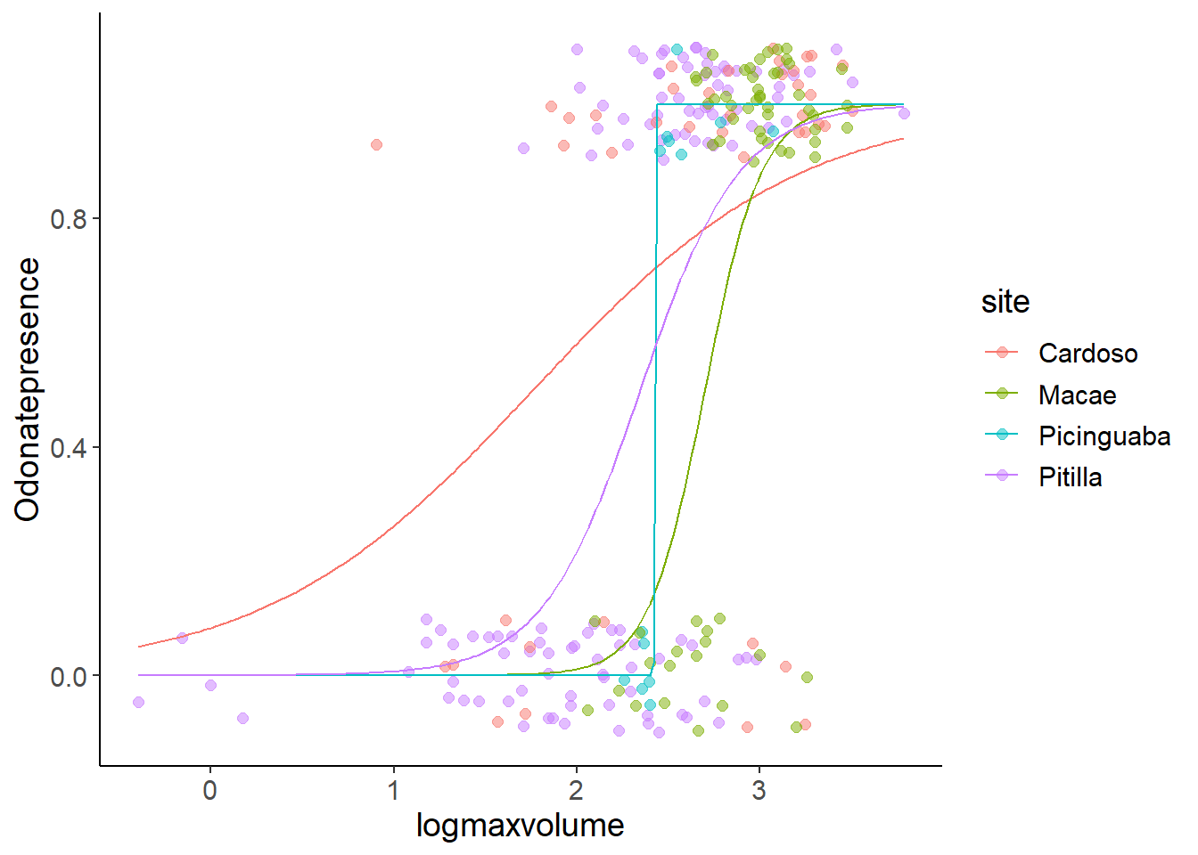

Now, we can see what is going on: In the site Picinguaba there is a sharp size threshold between small bromeliads without Odonata and bigger ones with Odonata. This extreme shape can be fitted with arbitrarily small intercepts and arbitrarily high slope values, which causes the uncertainty in the parameter estimates.

When we want to avoid this, we can use a model without the interaction:

model3 <- glm(Odonatepresence ~ logmaxvolume + site,
                  family = binomial, data = bromeliads)

drop1(model3, test = "Chi")

Single term deletions

Model:
Odonatepresence ~ logmaxvolume + site
             Df Deviance    AIC    LRT Pr(>Chi)    
<none>            219.27 229.27                    
logmaxvolume  1   304.96 312.96 85.688  < 2e-16 ***
site          3   226.57 230.57  7.296  0.06303 .  
---
Signif. codes:  0 '***' 0.001 '**' 0.01 '*' 0.05 '.' 0.1 ' ' 1

summary(model3)

Call:
glm(formula = Odonatepresence ~ logmaxvolume + site, family = binomial, 
    data = bromeliads)

Coefficients:
               Estimate Std. Error z value Pr(>|z|)    
(Intercept)     -6.5689     1.1562  -5.682 1.33e-08 ***
logmaxvolume     3.1594     0.4603   6.864 6.68e-12 ***
siteMacae       -1.5967     0.6473  -2.467   0.0136 *  
sitePicinguaba  -1.1448     0.7773  -1.473   0.1408    
sitePitilla     -0.8239     0.5636  -1.462   0.1437    
---
Signif. codes:  0 '***' 0.001 '**' 0.01 '*' 0.05 '.' 0.1 ' ' 1

(Dispersion parameter for binomial family taken to be 1)

    Null deviance: 316.07  on 233  degrees of freedom
Residual deviance: 219.27  on 229  degrees of freedom
AIC: 229.27

Number of Fisher Scoring iterations: 5

pred_dat$pred_prob_3 <- predict(model3, newdata = pred_dat, type = "response")

ggplot(bromeliads, aes(x = logmaxvolume, y = Odonatepresence, color = site)) +
  geom_jitter(height = 0.1, width = 0, size = 2, alpha = 0.5) +
  geom_line(aes(logmaxvolume, pred_prob_3), data = pred_dat)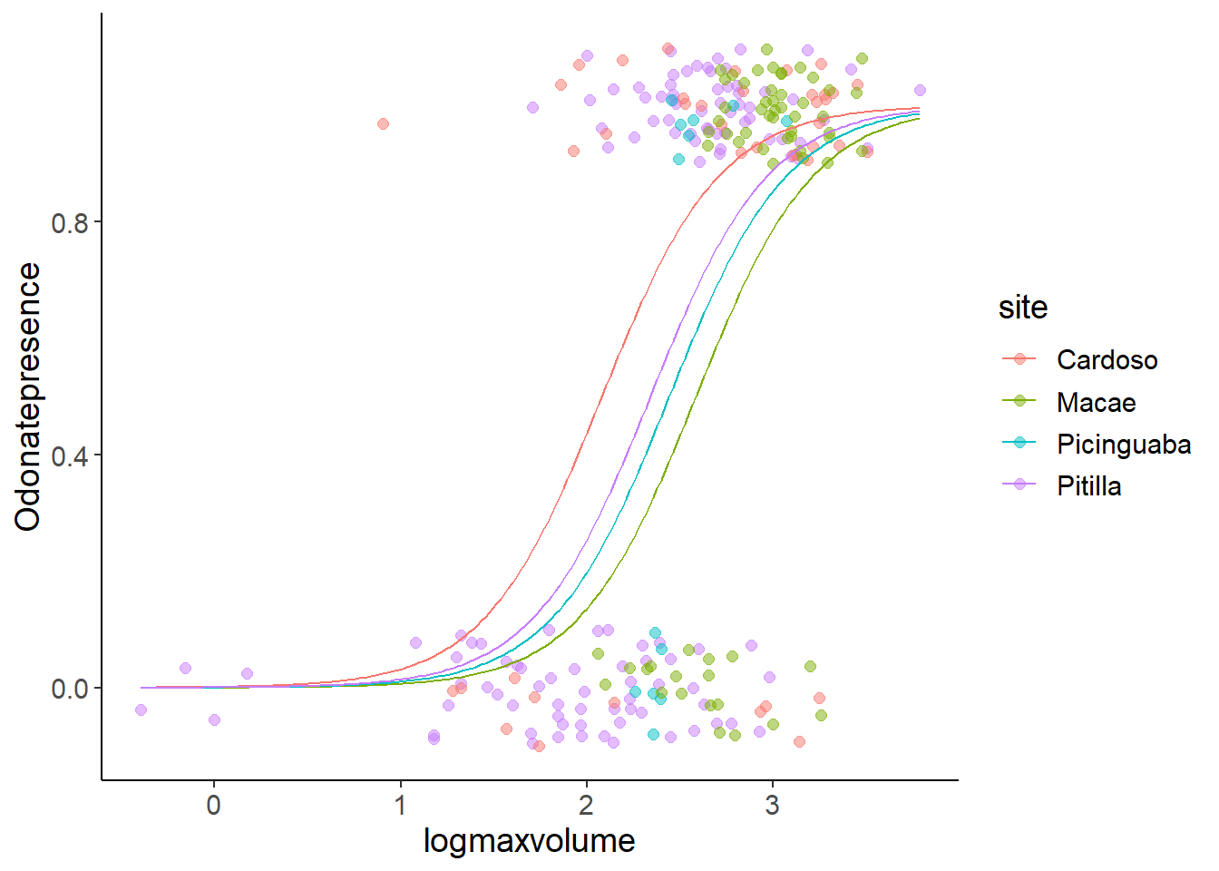

This model indicates that the different intercepts between the sites are only marginally significant in the output of drop1(). At the same time, we can properly estimate the values of the model parameters.

In such a case, there is no clear answer if we should prefer model2 with the significant interaction, but uncertain parameter estimates, or the model3 with certain parameter estimates, but with little evidence for any differences between sites. What we do and argue in this case will depend on the question that we want to answer. Potentially, collecting more data in Picinguaba might be an option to avoid the sharp threshold.

2 Solution as one script without output

library(readr)
library(ggplot2)
library(dplyr)
library(tidyr)

## theme for ggplot
theme_set(theme_classic())
theme_update(text = element_text(size = 14))

# Read and plot the data
bromeliads <- read_csv("data/08_bromeliads.csv")

ggplot(bromeliads, aes(x = logmaxvolume, y = Odonatepresence)) +
  geom_point()

# Add jitter
ggplot(bromeliads, aes(x = logmaxvolume, y = Odonatepresence)) +
  geom_jitter(height = 0.1, width = 0, size = 2, alpha = 0.5) 

# Fit model
model1 <- glm(Odonatepresence ~ logmaxvolume,
              family = binomial(link = "logit"),
              data = bromeliads)

# Test effect of logmaxvolume
drop1(model1, test = "Chi")

# Look at direction of effect
summary(model1)

# Create and plot predictions
min_vol <- min(bromeliads$logmaxvolume)
max_vol <- max(bromeliads$logmaxvolume)

odonate_pred <- tibble(logmaxvolume = seq(min_vol,
                                          max_vol,
                                          length = 200))
odonate_pred$pred <- predict(model1, newdata = odonate_pred,
                             type = "response")

ggplot(bromeliads, aes(x = logmaxvolume, y = Odonatepresence)) +
  geom_jitter(height = 0.1, width = 0, size = 2, alpha = 0.5)  +
  geom_line(aes(logmaxvolume, pred), data = odonate_pred,
            color = "red")

# Extra -----------------------------------------------

# Fit and check model
model2 <- glm(Odonatepresence ~ logmaxvolume * site,
                  family = binomial, data = bromeliads)
drop1(model2, test = "Chi")
summary(model2)

# Create and plot predictions
pred_dat <- expand_grid(logmaxvolume = seq(min_vol,
                                           max_vol,
                                          length = 200),
                        site = unique(bromeliads$site))
pred_dat$pred_prob <- predict(model2, newdata = pred_dat, type = "response")

# Also use a model without interactions to avoid the problems in parameter 
# estimation
model3 <- glm(Odonatepresence ~ logmaxvolume + site,
                  family = binomial, data = bromeliads)

drop1(model3, test = "Chi")

summary(model3)

pred_dat$pred_prob_3 <- predict(model3, newdata = pred_dat, type = "response")

ggplot(bromeliads, aes(x = logmaxvolume, y = Odonatepresence, color = site)) +
  geom_jitter(height = 0.1, width = 0, size = 2, alpha = 0.5) +
  geom_line(aes(logmaxvolume, pred_prob_3), data = pred_dat)