library(readr)
library(ggplot2)
library(dplyr)
library(tidyr)

## theme for ggplot
theme_set(theme_classic())
theme_update(text = element_text(size = 14))Solution for prairiedog example
1 Solution with R output
Preparations
Load packages
Read data and calculate proportions
pdogs1 <- read_csv("data/08_prairiedogs.csv")

pdogs1 <- pdogs1 %>%
  mutate(n.surv = n.tot - n.death,
         p.surv = n.surv / n.tot
  )
1.1 Graphical data exploration
1.1.1 Two-way interactions
ggplot(pdogs1, aes(hibernation, p.surv, fill = mated)) +
  geom_boxplot()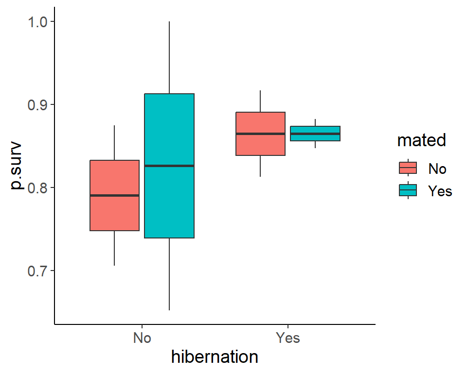
ggplot(pdogs1, aes(min.weight, p.surv, fill = mated)) +
  geom_boxplot()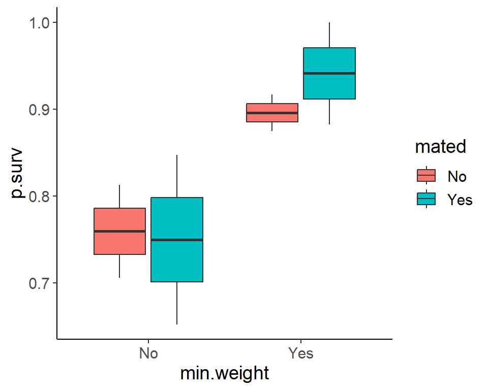
ggplot(pdogs1, aes(min.weight, p.surv, fill = hibernation)) +
  geom_boxplot()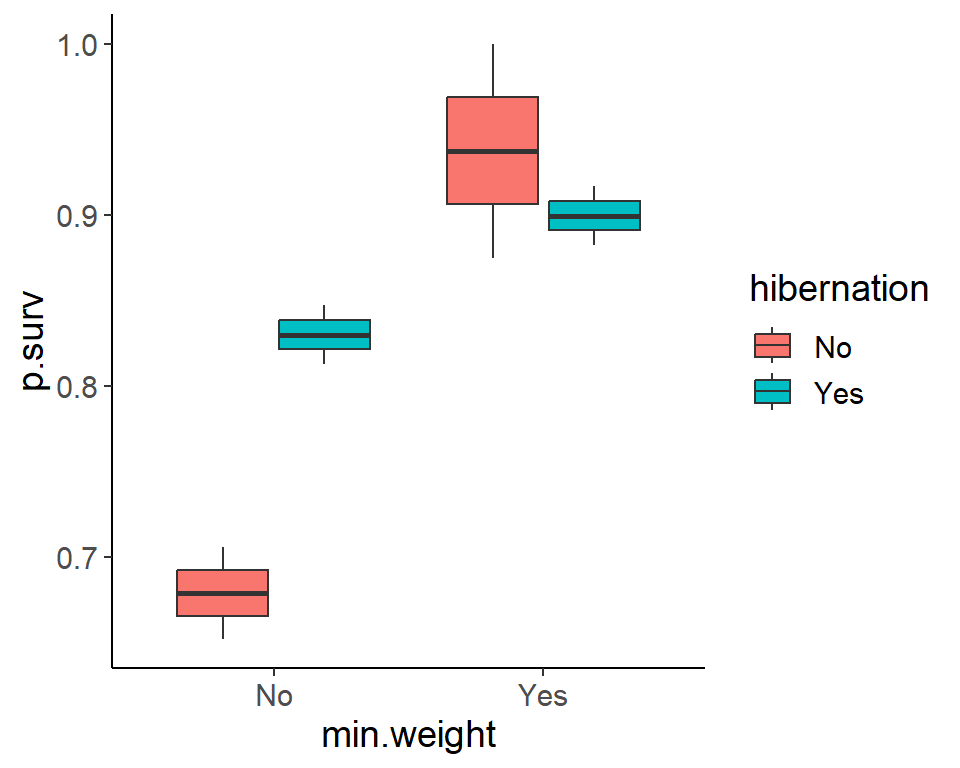
1.1.2 Main effects
ggplot(pdogs1, aes(mated, p.surv)) +
  geom_boxplot()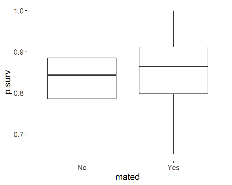
ggplot(pdogs1, aes(hibernation, p.surv)) +
  geom_boxplot()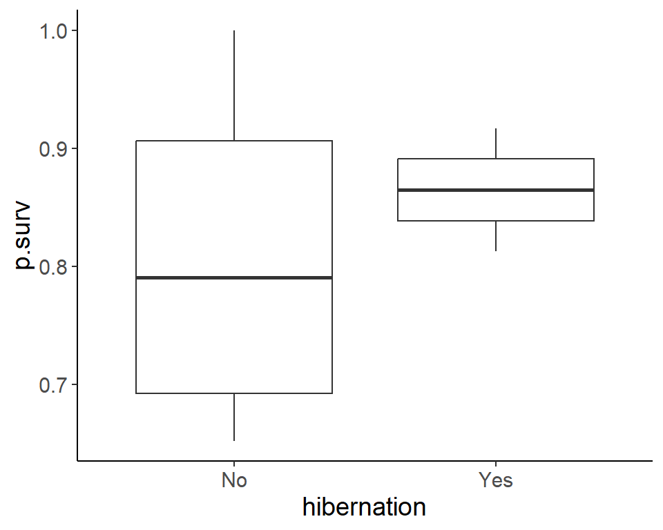
ggplot(pdogs1, aes(min.weight, p.surv)) +
  geom_boxplot()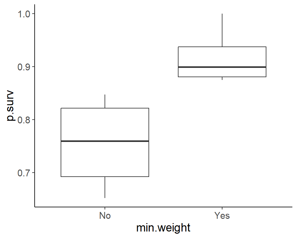
1.2 Model with two-way interactions
1.2.1 Fit the model
model1 <- glm(cbind(n.surv, n.death) ~ mated + hibernation + min.weight +
                mated:hibernation + mated:min.weight + hibernation:min.weight,
              family = binomial, data = pdogs1)
1.2.2 Test the two-way interactions
drop1(model1, test = "Chi")Single term deletions
Model:
cbind(n.surv, n.death) ~ mated + hibernation + min.weight + mated:hibernation +
mated:min.weight + hibernation:min.weight
Df Deviance AIC LRT Pr(>Chi)
<none> 0.82565 39.744
mated:hibernation 1 1.18134 38.100 0.35569 0.5509
mated:min.weight 1 0.97217 37.891 0.14651 0.7019
hibernation:min.weight 1 1.13001 38.049 0.30436 0.5812No evidence at all for any clear interaction.
1.3 Model with main-effects only
1.3.1 Fit the model
model2 <- glm(cbind(n.surv, n.death) ~ mated + hibernation + min.weight,
              family = binomial, data = pdogs1)
1.3.2 Test the main effects
drop1(model2, test = "Chi")Single term deletions
Model:
cbind(n.surv, n.death) ~ mated + hibernation + min.weight
Df Deviance AIC LRT Pr(>Chi)
<none> 1.6184 34.537
mated 1 1.6781 32.597 0.0597 0.80694
hibernation 1 7.2750 38.194 5.6566 0.01739 *
min.weight 1 7.2963 38.215 5.6779 0.01718 *
---
Signif. codes: 0 '***' 0.001 '**' 0.01 '*' 0.05 '.' 0.1 ' ' 1Hibernation and min.weight seems to have a significant association with survival.
1.4 Extra
For the predictions, we create a model which includes the significant explanatory variables only and use this model to predict the survival probabilities for all combinations of hibernation and minimum weight.
We show the predicted values as points.
model3 <- glm(cbind(n.surv, n.death) ~
              min.weight + hibernation,
            data = pdogs1, family = "binomial")

pred_dat <- expand_grid(hibernation = unique(pdogs1$hibernation),
                        min.weight  = unique(pdogs1$min.weight))

pred_dat$p_surv_pred <- predict(model3, type = "response", newdata = pred_dat)

ggplot(pdogs1, aes(x = hibernation, y = p.surv,
                   fill = min.weight)) +
  geom_boxplot() +
  geom_point(aes(y = p_surv_pred),
             data = pred_dat,
             position = position_dodge(width = 0.75),
             shape = 21, size = 5, show.legend = F) +
ylab("Proportion survivors") 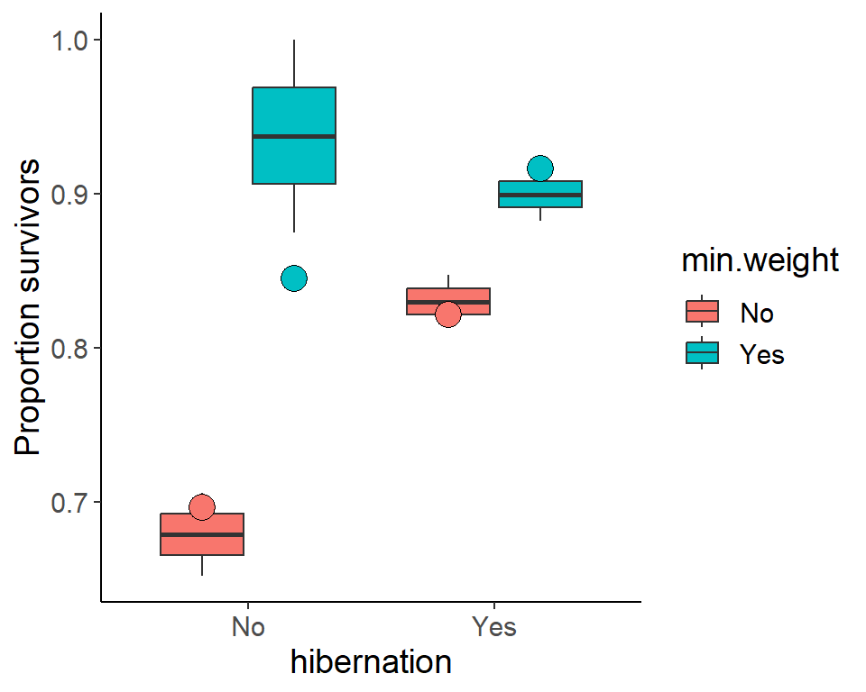
Finally, we check if using the proportion of survivors as response and the total number of prairie dogs for each combination as weights leads to the same results. As example, we do this with the model with all main effects here, but it should be the same for all other models as well.
# Model with proportion plus weights as comparison
model2a <- glm(p.surv ~ mated + hibernation + min.weight,
              family = binomial, data = pdogs1,
              weights = n.tot)

# The summaries should be exactly the same
summary(model2a)
Call:
glm(formula = p.surv ~ mated + hibernation + min.weight, family = binomial,
    data = pdogs1, weights = n.tot)

Coefficients:
               Estimate Std. Error z value Pr(>|z|)
(Intercept)     0.81041    0.25902   3.129  0.00176 **
matedYes        0.06777    0.27812   0.244  0.80747
hibernationYes  0.69531    0.28509   2.439  0.01473 *
min.weightYes   0.87194    0.39757   2.193  0.02830 *
---
Signif. codes:  0 '***' 0.001 '**' 0.01 '*' 0.05 '.' 0.1 ' ' 1

(Dispersion parameter for binomial family taken to be 1)

    Null deviance: 14.1259  on 7  degrees of freedom
Residual deviance:  1.6184  on 4  degrees of freedom
AIC: 34.537

Number of Fisher Scoring iterations: 4summary(model2)
Call:
glm(formula = cbind(n.surv, n.death) ~ mated + hibernation +
    min.weight, family = binomial, data = pdogs1)

Coefficients:
               Estimate Std. Error z value Pr(>|z|)
(Intercept)     0.81041    0.25902   3.129  0.00176 **
matedYes        0.06777    0.27812   0.244  0.80747
hibernationYes  0.69531    0.28509   2.439  0.01473 *
min.weightYes   0.87194    0.39757   2.193  0.02830 *
---
Signif. codes:  0 '***' 0.001 '**' 0.01 '*' 0.05 '.' 0.1 ' ' 1

(Dispersion parameter for binomial family taken to be 1)

    Null deviance: 14.1259  on 7  degrees of freedom
Residual deviance:  1.6184  on 4  degrees of freedom
AIC: 34.537

Number of Fisher Scoring iterations: 4
2 Solution as one script without output
library(readr)
library(ggplot2)
library(dplyr)
library(tidyr)

pdogs1 <- read_csv("data/08_prairiedogs.csv")

pdogs1 <- pdogs1 %>%
  mutate(n.surv = n.tot - n.death,
         p.surv = n.surv / n.tot
  )

# 1. Graphical data exploration

# 1.1 Create appropriate figures to explore all potential two-way interactions.
ggplot(pdogs1, aes(hibernation, p.surv, fill = mated)) +
  geom_boxplot()

ggplot(pdogs1, aes(min.weight, p.surv, fill = mated)) +
  geom_boxplot()

ggplot(pdogs1, aes(min.weight, p.surv, fill = hibernation)) +
  geom_boxplot()

# 1.2 Create appropriate figures to explore all potential main effects.
ggplot(pdogs1, aes(mated, p.surv)) +
  geom_boxplot()

ggplot(pdogs1, aes(hibernation, p.surv)) +
  geom_boxplot()

ggplot(pdogs1, aes(min.weight, p.surv)) +
  geom_boxplot()


# 2. Model and test all possible two-way interactions

# 2.1 Fit a model with all main effects and all two-way interactions
model1 <- glm(cbind(n.surv, n.death) ~ mated + hibernation + min.weight +
                mated:hibernation + mated:min.weight + hibernation:min.weight,
              family = binomial, data = pdogs1)

# 2.2 Test the two-way interactions using Likelihood-Ratio-Tests
drop1(model1, test = "Chi")

# 3. Model and test the main effects

# 3.1 Fit a model with all main effects
model2 <- glm(cbind(n.surv, n.death) ~ mated + hibernation + min.weight,
              family = binomial, data = pdogs1)

# 3.2 Test the main effects using Likelihood-Ratio-Tests
drop1(model2, test = "Chi")

# Extra ----------------------------------------------------------------------

# Figure with predictions
model3 <- glm(cbind(n.surv, n.death) ~
              min.weight + hibernation,
            data = pdogs1, family = "binomial")

pred_dat <- expand_grid(hibernation = unique(pdogs1$hibernation),
                        min.weight  = unique(pdogs1$min.weight))

pred_dat$p_surv_pred <- predict(model3, type = "response", newdata = pred_dat)

ggplot(pdogs1, aes(x = hibernation, y = p.surv,
                   fill = min.weight)) +
  geom_boxplot() +
  geom_point(aes(y = p_surv_pred),
             data = pred_dat,
             position = position_dodge(width = 0.75),
             shape = 21, size = 5, show.legend = F) +
             ylab("Proportion survivors")

# Model with proportion plus weights as comparison
model2a <- glm(p.surv ~ mated + hibernation + min.weight,
              family = binomial, data = pdogs1,
              weights = n.tot)

# The summaries should be exactly the same
summary(model2a)
summary(model2)
model3 <- glm(cbind(n.surv, n.death) ~
min.weight + hibernation,
data = pdogs1, family = "binomial")
pdogs1$p_surv_pred <- predict(model3, type = "response")
ggplot(pdogs1, aes(x = hibernation, y = p.surv,
fill = min.weight)) +
geom_boxplot() +
geom_point(aes(y = p_surv_pred),
position = position_dodge(width = 0.75),
shape = 21, size = 5, show.legend = F) +
ylab("Proportion survivors") 