Solution for exercise on browsing damage on tree saplings

1 Preparations

• Loading required packages and set ggplot theme.

library(readr)
library(ggplot2)
library(dplyr)
library(tidyr)

## theme for ggplot
theme_set(theme_classic())
theme_update(text = element_text(size = 14))

2 Read the data

dat_browse <- read_csv("data/09_dataset2_tree_browsing.csv")
dat_browse

# A tibble: 179 × 4
   canopy_closure species N_browsed N_total
            <dbl> <chr>       <dbl>   <dbl>
 1             78 Acer           10      23
 2             78 Fagus          12      55
 3             78 Picea           1      15
 4             61 Acer           20      31
 5             61 Fagus           6      13
 6             61 Picea           3      40
 7             69 Acer           19      55
 8             69 Fagus          17      41
 9             69 Picea           1      46
10             73 Acer           25      50
# ℹ 169 more rows

3 Graphical data exploration

We are interested in the proportion of browsed sapling, so we calculate this first:

dat_browse <- dat_browse %>%
  mutate(prop_browsed = N_browsed/N_total)

Now, we can plot the relationship of tthe two explanatory variables with the proportion of browsed saplings:

ggplot(dat_browse, aes(canopy_closure, prop_browsed, color = species)) +
  geom_point()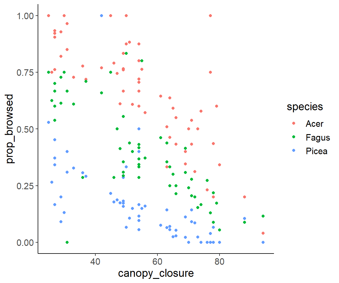 

We can “guesstimate” that rowdeer like Acer best and Picea least. Furthermore, browsing might decrease with canopy closure, but of course these guesses should be tested with statistics.

4 Statistical modelling

4.1 Fitting the first model

Since we have proportion data here, we chose a GLM with binomial distribution and logit link function as model. Note the response variable with two columns, which are the no. of browsed sapling and the no. of unbrowsed saplings.

glm1 <- glm(cbind(N_browsed, N_total - N_browsed) ~ canopy_closure*species,
            data = dat_browse, family = "binomial")
summary(glm1)

Call:
glm(formula = cbind(N_browsed, N_total - N_browsed) ~ canopy_closure * 
    species, family = "binomial", data = dat_browse)

Coefficients:
                             Estimate Std. Error z value Pr(>|z|)    
(Intercept)                  3.665267   0.242568  15.110  < 2e-16 ***
canopy_closure              -0.054936   0.003972 -13.832  < 2e-16 ***
speciesFagus                -1.587928   0.309384  -5.133 2.86e-07 ***
speciesPicea                -2.891099   0.327896  -8.817  < 2e-16 ***
canopy_closure:speciesFagus  0.008344   0.005224   1.597    0.110    
canopy_closure:speciesPicea  0.003982   0.006236   0.639    0.523    
---
Signif. codes:  0 '***' 0.001 '**' 0.01 '*' 0.05 '.' 0.1 ' ' 1

(Dispersion parameter for binomial family taken to be 1)

    Null deviance: 1491.08  on 178  degrees of freedom
Residual deviance:  192.27  on 173  degrees of freedom
AIC: 719.83

Number of Fisher Scoring iterations: 4

There is no indication of overdispersion (192.27/173 = 1.11) so we do not need to account for it and can test the interaction

test1 <- drop1(glm1, test = "Chi")
test1

Single term deletions

Model:
cbind(N_browsed, N_total - N_browsed) ~ canopy_closure * species
                       Df Deviance    AIC    LRT Pr(>Chi)
<none>                      192.27 719.83                
canopy_closure:species  2   194.85 718.41 2.5852   0.2746

The interaction is not supported so we also fit a model with the both main effects only.

glm2 <- glm(cbind(N_browsed, N_total - N_browsed) ~ canopy_closure + species,
            data = dat_browse, family = "binomial")
test2 <- drop1(glm2, test = "Chi")
test2

Single term deletions

Model:
cbind(N_browsed, N_total - N_browsed) ~ canopy_closure + species
               Df Deviance     AIC    LRT  Pr(>Chi)    
<none>              194.85  718.41                     
canopy_closure  1   781.51 1303.07 586.66 < 2.2e-16 ***
species         2  1101.65 1621.21 906.80 < 2.2e-16 ***
---
Signif. codes:  0 '***' 0.001 '**' 0.01 '*' 0.05 '.' 0.1 ' ' 1

The main effects have very strong statistical support. Clearly, this finding will not be changed by p-value adjustment because of multiple testing, but for completeness I show it here again:

4.2 P-value adjustment because of multiple testing

p_vals <- c(test1$`Pr(>Chi)`[2], test2$`Pr(>Chi)`[2:3])
p_vals

[1]  2.745551e-01 1.333463e-129 1.230754e-197

As expected the two p-values for the main effects are essentially zero. So we have strong evidence that canopy closure has an effect on browsing and species differ in their browsing.

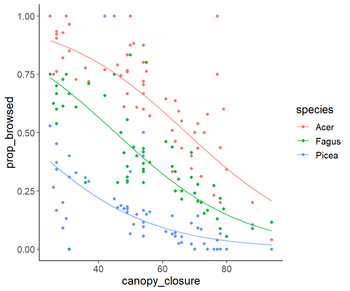
5 Create and plot predictions

Finally, we plot the data together with the predictions of the model with the two main effects.

As usual, we first generate new data for predictions:

pred_dat <- expand_grid(canopy_closure = seq(min(dat_browse$canopy_closure),
                                             max(dat_browse$canopy_closure),
                                             length = 100),
                        species = unique(dat_browse$species))

pred_dat$pred_pi <- predict(glm2, pred_dat, type = "response")

And then we can plot everything:

ggplot(dat_browse, aes(canopy_closure, prop_browsed, color = species)) +
  geom_point() +
  geom_line(aes(y = pred_pi), data = pred_dat)